Chapter 2. Introduction

Scream! 4.6 is a software application for seismometer configuration, real-time acquisition and monitoring. It runs on Linux and Windows (from 98 onwards) on both 32-bit and 64-bit PCs. It can be used for decompressing, viewing, printing, recording, transmitting and replaying GCF data from any Güralp Systems digital device.

Scream! 4.6 can be used in two modes:

• as a stand-alone, real time application for real-time data acquisition, including a network server and client, file replay, recording and analysis tools; or

• as a “helper” application for viewing pre-recorded GCF files. This mode also allows you to convert data formats and launch analysis tools.

2.1 Scream! as a real time application

When you run Scream! by double-clicking on its icon, or by launching it from the command line, it opens a Main Window showing all of the data streams coming in.

Scream! can listen for incoming streams in GCF format on local serial ports or network interfaces, as well as actively requesting data from network sources.

The Main Window is the control centre for the whole program. If you close this window, Scream! will quit. All of Scream!'s functions are invoked from this window: see Chapter 5 for details.

You can view a data stream by opening a WaveView window for it. Any number of WaveView windows can be opened, each containing any number of streams. The same stream can appear in several WaveView windows, if desired. Each WaveView window has its own amplitude and time scaling, colour scheme, and display parameters. For example:

• a single data stream can be viewed simultaneously at different zoom factors in different windows;

• different groups of data streams can be viewed simultaneously, each group having the same zoom factor; or

• an entire array can be monitored in one window, using another window for detailed examination of incoming data.

WaveView windows provide simple filtering capabilities, allowing you to examine seismic signals within a particular frequency range of interest. When more detailed analysis is required, data can be passed to a configurable range of Scream! extensions with a simple, mouse-driven selection process.

WaveView windows are fully described in Chapter 6; Scream! extensions are covered in Chapter 14.

2.1.1 Diagnostic features

Scream! performs extensive checks on all incoming GCF data and logs any errors to disk. You can see details about the incoming data, including any errors detected by Scream!, using the ShowInfo, Network Control, Summary and Status windows. These are described in Chapter 8.

Scream! also provides logging facilities and can e-mail operators when a potential problem is detected, as described in Chapter 13.

2.1.2 Digitiser configuration

Scream! provides an easy-to-use graphical interface for configuring Güralp DM24 and CD24 digitisers, including in digital instruments such as the 3TD and 6TD. Output stream selection, triggering, calibration and mass control can all be managed by Scream!.

See Chapter 9 and Chapter 10 for more information on these features.

2.1.3 Networking

The real time Scream! application provides a built-in network server and client for data in GCF format. A Network Control window provides full control of Scream!'s network connections. The Scream! server can be configured to allow remote clients to configure digitisers and control instruments over the network.

Client functions (data acquisition) are described in section 4.3 while Chapter 7 describes Scream!'s server functions.

2.1.4 Recording and replay

Scream! can record data to disk in a variety of formats. Scream! supports GCF, SAC, miniSEED, P-SEGy, SEG2, PEPP, SUDs and GSE, among others, allowing you to transfer data quickly and easily for further analysis or processing. Recorded files can optionally be post-processed by your own scripts or programs; either for file-transfer or data transformation.

GCF data files, including data from Güralp Systems NAM, Affinity or EAM units, can be read, replayed at variable time-scales, viewed, converted or printed with a few mouse clicks.

Support for SCSI tape devices is also included for accessing historical archives.

See Chapter 11 and Chapter 12 for details of these features.

2.2 Scream! as a data viewer

Scream! can be run in a slimmed-down viewing mode, which loads in a GCF file, a selection of GCF files, or an entire directory tree containing GCF files, and displays the data in a WaveView window.

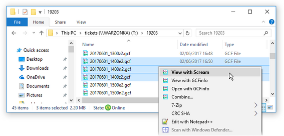
To use these features on a Windows PC, select one or more GCF files (or folders containing GCF files), right-click on the selection and, in the pop-up context menu that appears, click on the View in Scream entry to open a WaveView window showing the data in the file, files or folders.

Any valid GCF file can be loaded, including multi-stream files, files with gaps or out-of-order data and files containing status packets. If a file contains a mix of data and status packets, a WaveView will be opened for the data, and a status window for the status data.

WaveView windows opened this way behave exactly like windows from the real-time application, except that (i) the “pause” button ( ) is replaced with a button which resets the view to its initial settings ( ) and (ii) the original file is used instead of the Stream Buffer - see section 5.1 for a description of the Stream Buffer.

You can design and apply filters, plot spectrograms, or send data to Scream! extensions just as you would from real-time Scream!. See Chapter 6 for full details of the available options.

From the command line, Scream! can be run in viewing mode with

scream -view filename [filename…]

Scream! cannot transfer data between real-time mode and viewing mode. If you want to load GCF files into the real-time application, you should use the Replay Files facility (see section 11.2). However, you can have both real-time Scream! and Scream! viewer windows open at the same time.