Chapter 2. The example
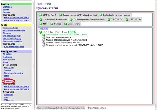
Start by selecting the “Triggering” option from the left-hand menu.
2.1 Calibration information
The first step is to enter calibration information for the instruments so that parameters can be entered in physical units, such as ms-2.
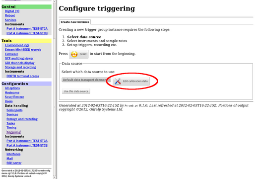
Click  and then
  :
:
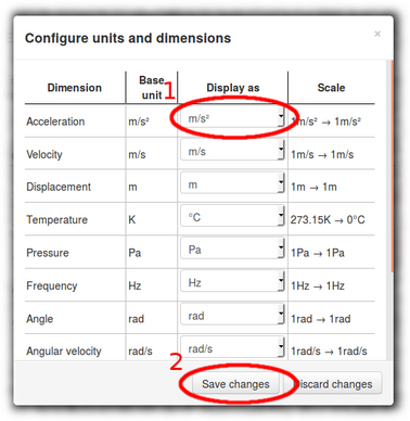
Specify your preferred units for each dimension that you intend to use and then click  . In this example, we choose m/s-2 as our preferred units for acceleration. These dimension units will be used throughout the remainder of the configuration process.
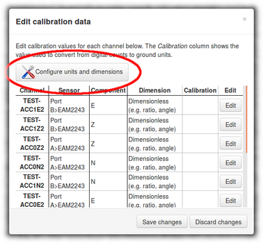
Next, specify the dimension (velocity, acceleration, etc.) and calibration values for each channel (ignoring unwanted channels). Click the  buttons to enter the information for each channel:
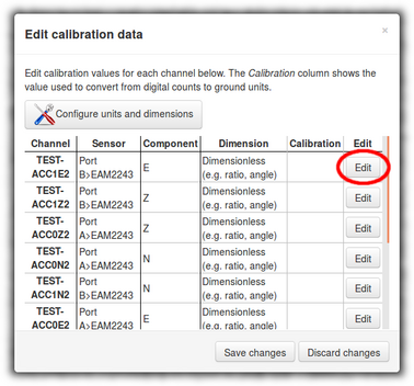
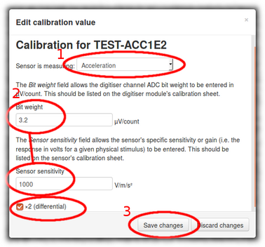
The basic measurement type - typically acceleration or velocity - should be specified at the top of the resulting screen. The values from the calibration sheets for both instrument and digitiser can be used to populate the rest of the fields. Click  when all the fields are correctly populated.
Repeat for each channel that you want to monitor or report on. Once calibration data for all channels have been entered, click
:

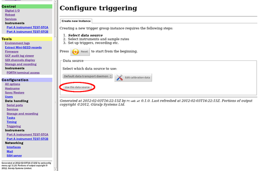
2.2 Data source
All but the most complex configurations will use the default data transport daemon (gdi-base), so click  to continue:
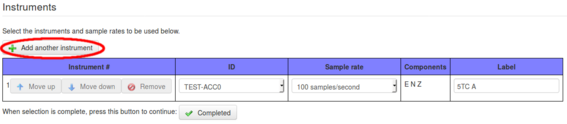
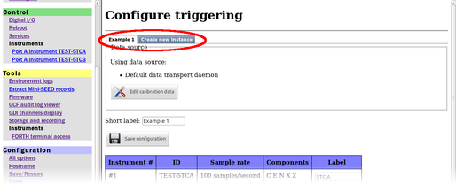
2.3 Instruments
Every combination of instrument and sample rate that will be used as a triggering source now needs to be listed in the “Instruments” section. They can be assigned labels that will be used in later dialogues.
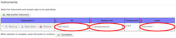
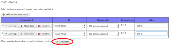
Click  to continue with the second sensor:
When all instruments have been listed, adjust the order if necessary using the  and
and  buttons. Unwanted instruments can be removed from this list with the
  button.
When finished, click  :
:
2.4 Trigger criteria
We now need to specify the criteria under which a trigger will be declared. Click  :
:
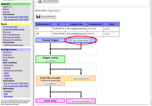
and select the trigger type:
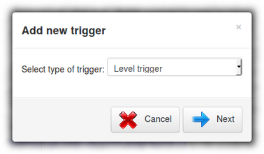
The possible types are:
Level trigger, where a trigger is declared if the absolute level of the input signal is greater than a specified threshold value; and
STA/LTA trigger, when the ratio of the short-term average (STA) to the long-term average (LTA) is monitored and a trigger declared if it passes a threshold. The periods over which the two averages are computed can be specified in the STA/LTA dialogue.
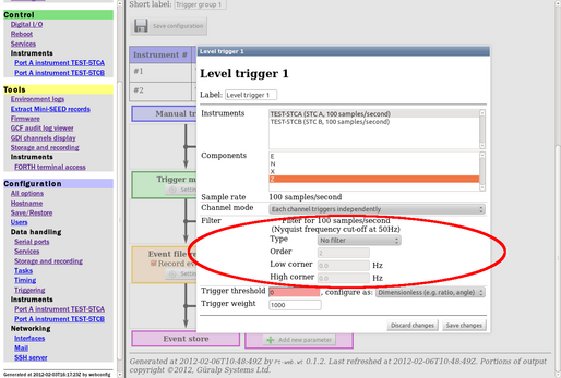
In both cases, facilities exist to filter the data before the calculations are carried out. This is highly advised: raw seismic data include inevitable offsets, which should be removed by an appropriate high-pass filter.
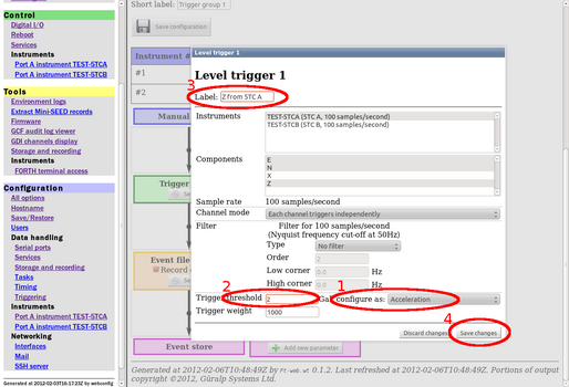
In this example, we will configure a level trigger. First, select the required instrument from the list by clicking on it:
Once the instrument is selected, it will appear highlighted. Pick the corresponding component or components to monitor:
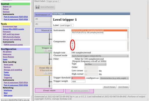
We will use just the vertical (Z) component for this example.
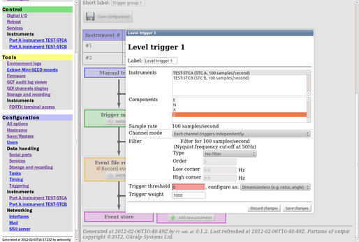
If multiple components are selected, you have the choice of declaring a trigger when any component exceeds the threshold or only when the resultant of all selected components exceeds the threshold.
It is recommended that a high-pass filter is always used when configuring triggers. The dialogue offers a comprehensive selection of filter types, each with configurable parameters:
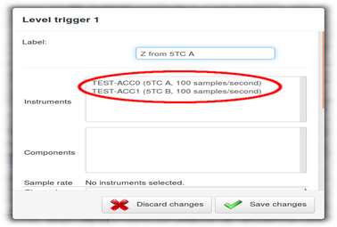
Next, choose the units for the threshold and specify the required value. Enter a label for this trigger and then click  . Note the trigger weight, 1000 (used when combining multiple triggers).
Click
again to add a second Level Trigger for the second instrument.
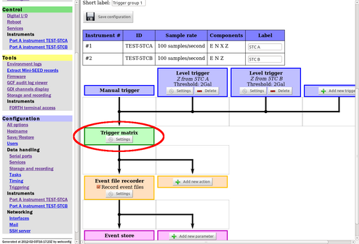
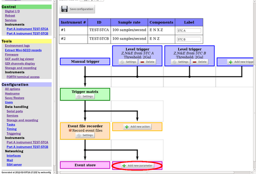
The two configured triggers will now appear side-by-side on the display, identified by the labels we specified earlier.
2.5 The trigger matrix
Next, click the  button for the Trigger matrix:
The resulting dialogue allows specification of the period of time for which a trigger remains valid. If another trigger occurs while the first is still valid, the two triggers are coalesced into a single trigger incident. This means that only a single event is declared and a single set of data are saved.
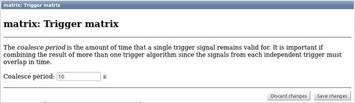
Data saved during a trigger include a pre-run period and a post-run period, which we will configure in the event file recorder dialogue. For coalesced triggers, the pre-run period is measured from the start of the first and the post-run period is measured from the end of the last.
Click  and then proceed to configure the Event file recorder.
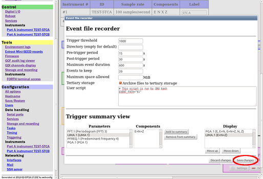
2.6 The Event file recorder
Click
to configure the Event file recorder.
We will revisit this dialogue later to compile a summary view but, for now, set the threshold to 1500. The weights of all active triggers must exceed this value for an event to be recorded. Our triggers had a weight of 1000 each, so a threshold of 1500 requires both to be active.
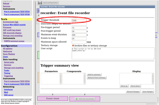
Click  and proceed to add parameters.
2.7 Parameters
Click  . We will use this to build a set of values to be recorded during an event.
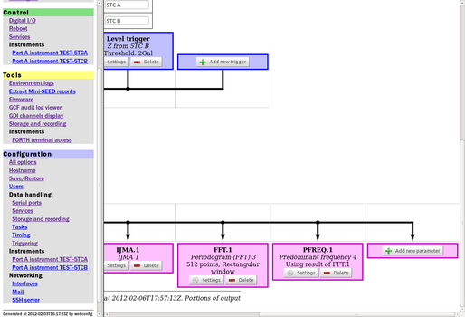
2.7.1 PGA
The first parameter we will add will be a PGA (peak ground acceleration). Select this from the drop-down menu:
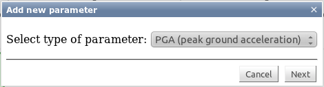
(The full list of options at the time of writing is:
PGA (peak ground acceleration)
IJMA (the earthquake intensity scale of the Japan Meteorological Agency)
Periodogram (fast Fourier transform); and
Predominant frequency (which takes its data from a periodogram which must, therefore, be configured first).
).
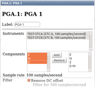
The following screen is displayed:
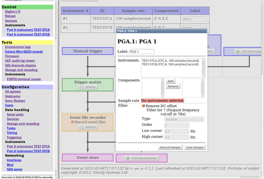
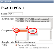
As before, we first select the instrument(s) that will be used as the data source. In this instance, we will use both instruments, so click the entry for the first instrument, then  +click the entry for the second. Both instruments will be highlighted and the components window will show all components available from all selected instruments; in this case, that will be E, N and Z.
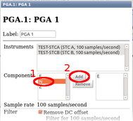
We now specify all of the required PGA calculations by selecting one or more components and clicking |
|
| |
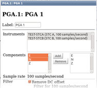
Start by selecting just the E component. When you click |

An 'E' appears in the right-hand box to indicate that the entries have been added. (You can remove an entry or entries if you make a mistake by highlighting them and clicking Add PGA calculations for the North components in a similar way: click “N” and then click |
| |
| The illustration to the left shows six single-component PGAs have been configured, three for each instrument. To add PGAs calculated from the two-dimensional resultant for each instrument, click “E” then | |
To add PGAs calculated from the three-dimensional resultant for each instrument, click “E” then |
| |
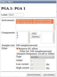
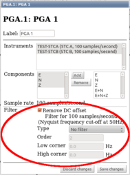
| It is possible to specify a filter which is applied to all components before they are used in the PGA calculation. Four different Butterworth types are available (high-pass, low-pass, band-pass and band-stop) and, for each, you can specify the order and the one or two corner frequencies. The “Remove DC offset” check-box enables a high-pass filter which works by subtracting the average of all samples from each sample in each packet. | |


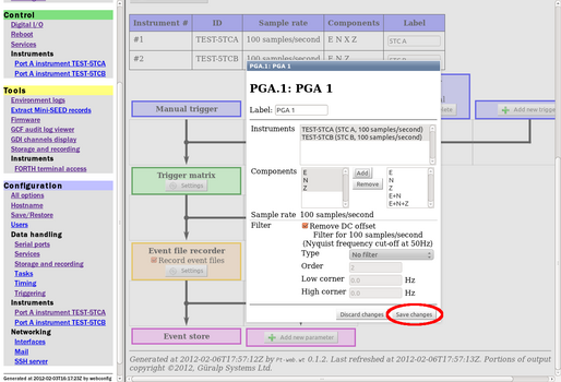
Once all the required PGAs have been specified (and a filter added if desired), you can add a descriptive label and then click  to close the PGA dialogue and continue. We will not bother with a label in this example because we only have one set of PGA calculations.
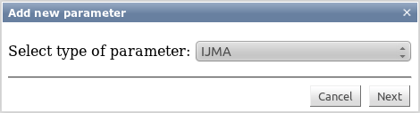
2.7.2 IJMA
Now click the  button again to to add an IJMA parameter. Select IJMA from the resulting drop-down menu:
As in previous screens, we are offered a dialogue from where we can select the instrument(s) that will serve as the data source and the component(s) that will be included in the calculation.
We will calculate two separate IJMAs, one for each instrument and both covering all three components. As before, this can all be specified in one dialogue.
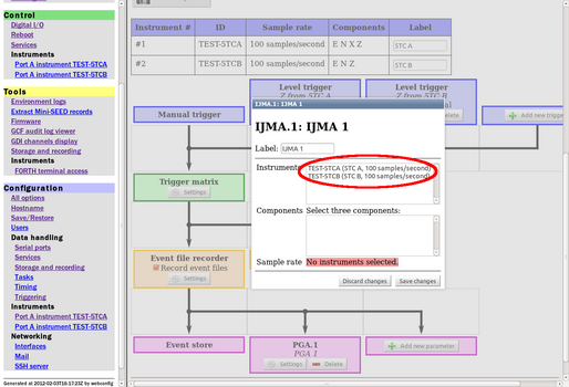
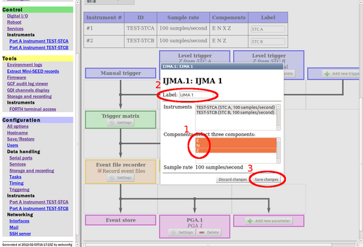
Click the entry for the first instrument, then  +click the entry for the second. Both instruments will be highlighted and the components window will show all components available from all selected instruments; in this case, that will be E, N and Z. Click the “E” component then
  +click the “N” and “Z” components. Add a label if desired and then click
:
+click the “N” and “Z” components. Add a label if desired and then click
:
2.7.3 Periodogram (FFT)
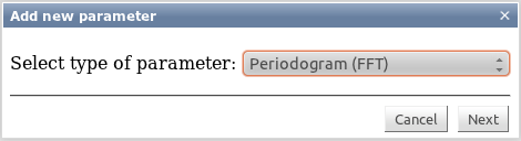
Next we will add a Periodogram so that we can compute a predominant frequency. Click
again and select “Periodogram (FFT)” from the drop-down menu:
As before, we select the required instrument / sample rate combinations. We will select both instruments and all three components (E, N & Z).
Click on the first instrument and then  +click the second instrument. When both are highlighted, click on the “E” component and then
  +click on the “N” and “Z” components.
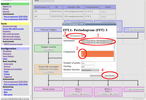
You can adjust the parameters of the FFT using the “Number of points”, “Overlap” and “Window function” parameters.
Enter a suitable label, if desired and then click
.
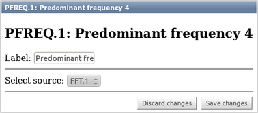
2.7.4 Predominant frequency
Next, we will add a predominant frequency parameter. Click
again and select “Predominant frequency” from the drop-down menu:

In the next dialogue, choose the FFT that we previously defined to use as the source and add an appropriate label before clicking  :
:
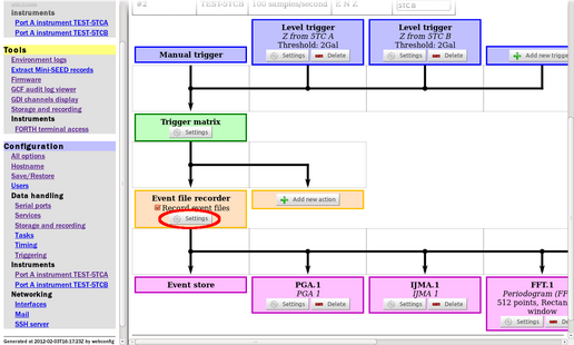
All the parameters that we have added now appear in a horizontal list:
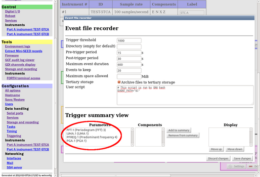
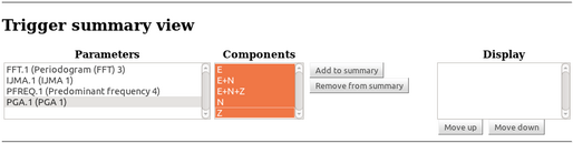
2.8 Trigger summary
To select which of these parameters to display when summarising a trigger event, scroll back to the left of the page and click the
button under “Event file recorder” again:
Select the desired parameters (and associated components) from the lists, then click  :
:
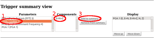
For our example, first click on PGA:
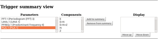
The list of available components appears. Click on the first and  +click the rest:
When all components are highlighted, click  . An entry will appear in the “Display” box.
Now repeat this for IJMA. Click on IJMA in the “Parameters” list, on “E+N+Z” in the “Components” list and then on  :
:
Once all of the desired parameters have been added, you can use the  and
and  buttons to adjust the order:
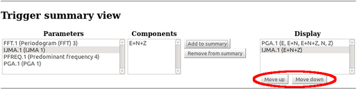
Once everything is in order, click
.
2.9 Saving
Finally, scroll back up the page and enter a practical name for this set of trigger settings and then click 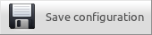 :
:
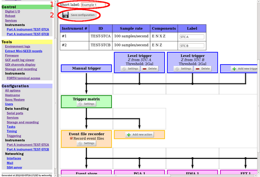
The next time that “Triggering” is selected from the “Configuration” menu, the dialogue will have tabs: The trigger group just created will be on the first tab and a “Create new instance” tab will allow you to set up a new trigger group if required. The new group would typically involve different instruments but this is not mandatory.
This completes the example. The Platinum Triggering subsystem is complex and has many features. We hope that this example has illustrated some of the ways in which the system can be used and given you confidence to explore the interface further as you develop your own configurations.