Chapter 3. Using the orientation sensor
3.1 Installing the sensor
The orientation sensor should be placed as near as possible to the head of the borehole. The sensor should be placed in an environment where the external interference from other sources will be small and where there is no direct sunlight. The sensor should be covered with a polystyrene box to reduce wind or convection noise sources.
Survey an accurate North/South line near the head of the borehole, and scribe it on a clean, solid horizontal surface. If the head of the borehole has a concrete surround, this is normally the best place to install the orientation sensor.
Loosen the retaining screw from the centre of the sensor base.
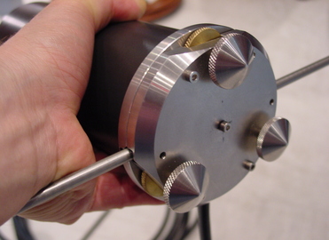
Thread the guide rod through the hole in the side of the sensor base. This rod is used to accurately help orient the sensor in the NORTH/SOUTH direction.
Re-tighten the retaining screw in the central hole to secure the guide rod to the instrument.
Mount the orientation sensor on the scribed North/South line.
The top panel of the orientation sensor includes a spirit level.
Level the sensor by adjusting the height of each foot in turn, until the bubble in the spirit level lies entirely within the inner circle. (The instrument can operate with up to 2 ° of tilt, but with reduced performance.)
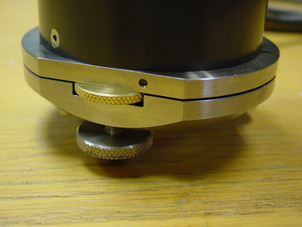
The feet are mounted on screw threads. To adjust the height of a foot, turn the brass locking nut anticlockwise (up) to loosen it, and rotate the foot so that it screws either in or out.
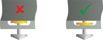
When you are happy with the height, tighten the brass locking nut clockwise (down) to secure the foot. When locked, the nut should be at the bottom of its travel for the best noise performance.
If the sensor moved off the scribed North/South line during levelling, carefully reposition it along the line. Make sure that the bubble in the spirit level remains within the inner circle. Level and reposition again if necessary.
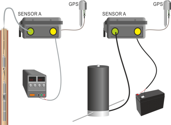
Connect the sensor signal cable to the Hand-held Control Unit. The orientation sensor power is supplied separately from the Hand-held Control Unit unit, as shown in the block diagrams in the following sections.
3.2 Installations with surface digitisers
3.2.1 DM24 mk3
Borehole installations using surface 3- or 6-channel DM24 mk3 digitisers are easily connected to the orientation kit with no additional hardware. These digitisers have an extra full-rate input channel which is exposed on pins on the AUXILIARY connector.
A Hand-held Control Unit (HCU) or Break-out Box (BoB) is required in order to unlock and centre the masses of the reference sensor.
The cabling between the Hand-held Control Unit and the AUXILIARY input of the digitiser is provided. This cable is labelled.
Because the two sensors are both connected to the same digitiser, they automatically share a common time base, so a GPS receiver is not strictly necessary.
DM24-based digitisers with more than 6 channels normally contain more than one internal digitiser module. For best results, you must ensure that the orientation sensor is connected to the same internal module as the borehole sensor.
To confirm the best configuration for your equipment, please contact Güralp Systems.
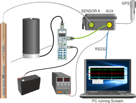
In this example, a PC or laptop is used to perform the orientation calculations on site. If this is impractical, the digitiser can be configured to store the experimental data and calculations can be performed later.
Using the cable provided (26-way plug to 19-way plug), connect the Hand-held Control Unit (or Break-out Box) to the AUXILIARY port of the digitiser.
Power the orientation sensor by connecting it to a 12 V battery using a suitable cable. The main power source for the rest of the installation can be used if practical but note that the orientation sensor is normally powered separately from the main installation to allow easy removal of the orientation kit after the experiment is finished.
Hold down the ENABLE switch on the Hand-held Control Unit, and press the LOCK/UNLOCK switch towards UNLOCK. Hold the two switches in this position for at least 6 seconds.
Note: The orientation sensor is wired such that the velocity output and the mass position output will appear on the Vertical (Z) channel on the Hand-held Control Unit.
The BUSY LED on the Hand-held Control Unit should light as the mass of the orientation sensor is unlocked, then flash as the mass is centred. When the BUSY LED goes out, the sensor is ready.
Installation is now complete: the remaining steps can be carried out remotely if required.
If necessary, use the digitiser to unlock the components of the borehole instrument.
Configure the digitiser to output data streams from the three components of the borehole instrument and the fourth auxiliary channel.
The microseismic peak occurs in the 0.1 – 1 Hertz frequency range, so a sample rate of 20 samples per second is generally sufficient.
The mass position of the orientation sensor is made available to the digitiser through the AUXILIARY port. It is exposed as Mux channel MB.
If you need this channel but it is not shown in Scream!, it may be disabled. In Scream's Configuration Setup window, choose the Mux channels pane and tick the MB box.
If you are using Scream!, check that seismic data are being received on all four channels.
Configure the installation to record this data, either in the Flash memory of your digitiser or on your computer using Scream!.
Leave the installation running for a period of time. The longer you can leave it, the more accurate the results will be. Running overnight, or longer, is strongly recommended, especially where diurnal cultural noise is expected.
Whilst the experiment is running, you should avoid introducing noise as much as possible. Noise generated by people moving around on the surface will be picked up by the reference sensor much more than the down-hole sensor. Since the experiment relies on the assumption that ground motion at the two sensors is similar, this will severely reduce the quality of data received.
If you have recorded data onto the DM24, transfer them to your PC using the DM24's FireWire interface or over a direct serial link.
The procedure for analysing these data is described in Section 3.4.
3.2.2 Affinity or DM24SxEAM
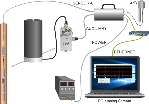
The procedure for using an Affinity or DM24SxEAM is essentially the same as that for the MD24 mk3, with the Auxiliary connector being used to provide an input for the fourth channel. Ethernet can be used instead of RS232, however.
3.2.3 Minimus
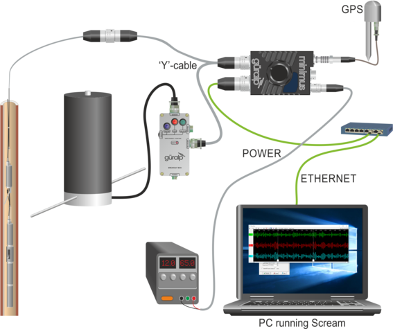
The auxiliary channel of a Minimus is exposed on the main analogue connector so, in this case, a 'Y'-cable is required so that the signals from both the borehole instrument and the reference sensor can be combined into a single cable.
The auxiliary channel of the Minimus appears in Scream as stream 0AUXX0.
3.3 Using a separate digitiser
The orientation calculation method described in this manual works best when the borehole sensor is digitised using the same time base as the reference sensor.
This is easily accomplished in the set-up above, because signals from the reference and borehole instruments are processed by a single unit. If you have the option, we recommend that you use a single digitiser in this way wherever possible.
However, it is also possible to perform an orientation experiment using a separate digitiser, relying on GPS to keep the time series synchronised.
Of course, if your borehole installation includes a down-hole digitiser, you will need to use a separate digitiser.
To do this:
Connect the orientation sensor directly to Port A of its digitiser. Power will be provided through the second digitiser rather than through a Hand-held Control Unit.
Alternatively, attach the HCU to the orientation sensor, and use a standard Güralp Systems 26-way sensor cable to connect this to PORT A.
Power the orientation sensor and the borehole installation.
Set up Scream! to receive data streams from both the borehole instrument and the orientation sensor.
Unlock the components of the borehole instrument and orientation sensor as necessary.
Configure the borehole installation to output data streams from all three components. Configure the surface digitiser to output the orientation sensor data stream.
The microseismic peak occurs in the 0.1 – 1 Hertz frequency range, so a sample rate of 20 samples per second is generally sufficient.
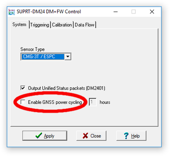
When recording orientation data from this type of installation, it is essential that both digitisers are permanently synchronised to GPS time. To ensure this, you should configure each digitiser to keep its GPS receiver powered at all times. In Scream!'s Configuration Setup window, this is done by clearing the Enable GPS power cycling check box.
Repeat this configuration on the other digitiser. Wait for a few minutes, and check that both digitisers have acquired a fix and reported a clock sync. When this happens, the top half of the digitiser's icon in Scream! will turn green
 .
.GPS information is also transmitted in the status stream of each digitiser. The message Clock sync'd to GPS indicates that the digitiser is synchronised.
When you run the experiment, you should allow at least 10 minutes before recording data, since both GPS systems will need to acquire a fix and synchronise their internal clocks.
The mass position of the orientation sensor is made available to the digitiser through the AUXILIARY port. It is exposed as Mux channel MB.
If you need this channel but it is not shown in Scream!, it may be disabled. In Scream's Configuration Setup window, choose the Mux channels pane and tick the MB box. (On older versions of Scream!, this box may be labelled Calibration Signal Input.)
If you are using Scream!, check that seismic data are being received on all four channels.
Configure the installation to record these data, either in the Flash memory of your digitiser, or on your computer using Scream!.
Leave the installation running for a period of time. The longer you can leave it, the more accurate the results will be. Running overnight, or longer, is recommended.
If you have recorded data into the Flash memory of either digitiser, transfer them to your PC by downloading directly, or using the DM24's FireWire interface.
3.4 Performing the analysis
Open the recorded files in Scream!. Under Windows, double-click on the .gcf files in Explorer. Under Linux, you can double-click on the files in Nautilus, Nemo etc if you have configured your system this way or, from the command line, you can run
scream --view path_to_.gcf_file
A WaveView window will open displaying your recorded streams:
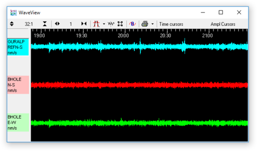
Drag the streams across the window so that the reference stream is at the top, the N stream in the middle, and the E stream at the bottom.
Locate a suitable data range. A good range would contain lots of teleseismic events and very little local noise. You should use a period of at least an hour, and preferably much longer.
Hold down
 and drag your mouse across the WaveView window with the left button held down until all three streams are selected for the whole range. Make sure there are no gaps in the data you select. If gaps are present in any streams, the selection for those streams will be shown with hatched lines to alert you:
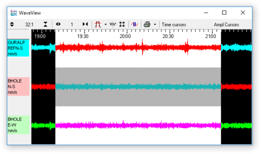
When you are happy with the selection, release the mouse button, but keep
held down.When the context menu appears, release the
key. Select Relative Orientation from the menu that appears.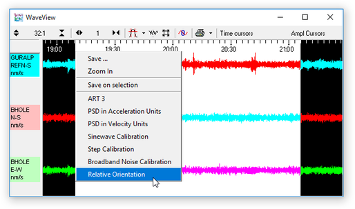
Two small windows will appear: a progress window and, typically, a warning with a legend like
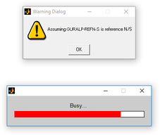
Scream! produces this warning when the reference sensor is not using a standard N/S channel, but the auxiliary (X) channel.
If you are using a separate digitiser, the warning will not appear.
If you see a different error message, make sure that the streams are in the correct order in the WaveView window. If you still have problems, you may have selected too few data points for it to be confident about the orientation; you should try again with a larger selection.
After a few seconds, the calculation should finish and three windows will appear. (Thye may obscure each other.)
The top window is a graph of Coherence vs Angle:
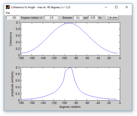
The two-stage algorithm rotates the N/S and E/W components of the sensor being tested in small steps.It measures first the amplitude similarity, and then the coherence between the virtual (rotated) N/S component and the reference N/S component, for a number of rotation angles.
The error in the final calculation is around 2.5°.
The peak of the coherence curve (upper graph) therefore corresponds to the angle of rotation which best matched the reference component. This angle is shown in the title bar, together with an estimated error.
You should see a coherence curve which is smooth and symmetrical. If the curve is distorted, either the surface data are too noisy or the data selection is too short.
The lower graph shows the overall amplitude similarity of the rotated signal. This provides an idea of the sign of the coherence (since signals in perfect antiphase have a high coherence as well as those in phase). If there are two peaks in the coherence graph, the correct one is where the amplitude similarity is most positive.
The sample plots show that the borehole instrument is installed with its N/S axis at a bearing of –90° from true North.
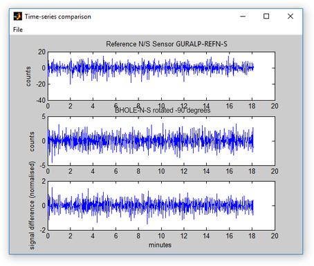
The second window shows the result of applying the rotation to the signal, i.e. the time series that a sensor in perfect N/S orientation would have produced:
You can perform more accurate calculations by narrowing the search range. This is done in the two left-hand-side entry boxes on the Coherence vs Angle window: the first denotes the centre of the new search and the second specifies its range.The program suggests suitable values for you, so in most cases you can just click
 to perform another iteration.
A new graph will be displayed showing the results.
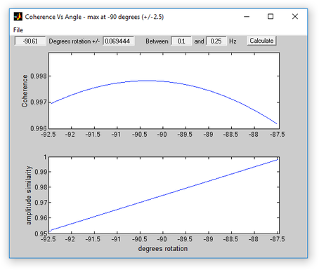
Our sample instrument is thus aligned at -90.61 ± 0.07°.
The error given is only a rough estimate. For best results, you should repeat the orientation experiment several times using different data sets. The true error in the computed orientation can then be determined by observing the spread of the results.
The Blacknest orientation method generally provides a reliable indication of the sensor's orientation. In most cases, the greatest source of error is in the installation of the reference sensor.
Note: If you have particular difficulty in deriving a stable value, additional information is contained in a third output window, which shows a waterfall plot of Coherence vs Frequency vs Angle. The frequency range used in the calculations is indicated with a black outline.
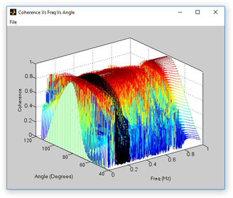
This plot can be used to select a more advantageous frequency range where the coherence curve is smoother and easier to interpret. In the example above, the frequency range 0.23 to 0.6 Hertz looks particularly promising: the surface within this range forms a smooth, symmetrical arch. Ideally, the peak should be very close to unity and the lowest points, at the margins, should be close to zero. The chosen frequency range can then be entered into the "Between X and Y Hz" boxes at the top of the "Coherence vs Angle" window before clicking  again; the data will be filtered accordingly before the coherence is recalculated, increasing the accuracy of the result.
3.5 Applying data rotations
Once you have determined the correct angle, you can program your digitiser to apply real-time mathematical rotations to the raw data. The procedure to do this is different for DM24 digitisers and Minimus digitisers. The DM24 procedure is described in the next section; the Affinity procedure is in section 3.5.2 on page 21 and the Minimus procedure is in section 3.5.3 on page 22.
3.5.1 DM24 digitisers
You can configure a DM24 mk3 digitiser to apply a rotation to the digitised data. It can then produce output streams representing ground motion on true North/South and East/West axes.
This is done within the DSP to minimize the reduction in data quality.
To set up the rotation:
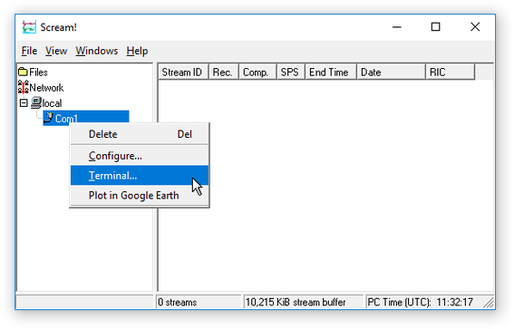
Open a terminal session with the digitiser. You can do this over a serial connection with a program such as minicom (for Linux) or PuTTY (for Microsoft Windows). If you have a serial connection to a PC running Scream!, you can access the digitiser's console by right-clicking on its icon and selecting Terminal....
Alternatively, if you access the DM24 via an EAM or other Platinum device, you can use the "FORTH Terminal Access" facility, reached via a web-page menu item , located under Tools→Terminal, or use the data-terminal tool from the command line.
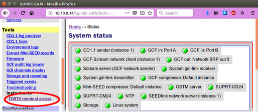
Regardless of the access method, you should see an ok prompt, indicating that the digitiser is ready to receive commands.
Type
0 rotation AZIMUTH
where rotation is the angle of deviation from true North that you measured earlier, as a whole number of tenths of a degree. This is the same angle as that given by the orientation program but with the opposite sign.
The 0 tells the digitiser to apply the rotation to instrument number 0 (the first, or only instrument.)
Thus in the example above, you would type 0 906 AZIMUTH to make the digitiser rotate signals by 90.6 degrees.
Reboot the digitiser with the command re-boot.
Collect some more data with the transformation active, and carry out another orientation calculation. The data from the down-hole instrument should now have a maximum coherence with the reference sensor at 0 °. Check in particular that the sign of the rotation you have applied is correct.
3.5.2 Affinity digitisers
The affinity digitiser can apply real-time rotation to its digitised data. It can then produce output streams representing ground motion on true North/South and East/West axes.
To configure this, visit the "Data acquisition" page of the web interface:
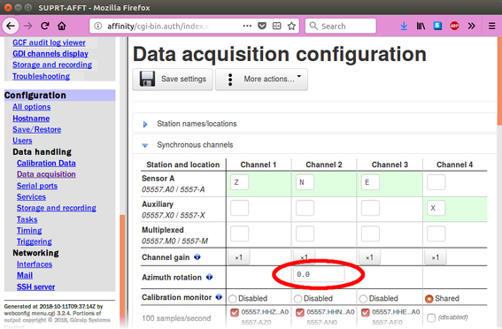
Enter the required angle - the sign-reversed output of the orientation calculations - into the "Azimuth rotation" field and then click  . (This feature assumes that the first three primary ADC channels are digitising the vertical, North/South and East/West components, respectively, of a triaxial digitiser.)
Once configured, collect some more data with the transformation active, and carry out another orientation calculation. The data from the down-hole instrument should now have a maximum coherence with the reference sensor at 0°. Check in particular that the sign of the rotation you have applied is correct.
3.5.3 Minimus digitisers
You can configure a Minimus digitiser to apply a real-time rotation to the digitised data. It can then produce output streams representing ground motion on true North/South and East/West axes.
The Minimus is capable of applying arbitrary three-dimensional rotations but we shall only use a single rotation about a vertical axis in this case. In the data-transform subsystem of the Minimus, rotations are specified using unit quaternions. This is a very flexible abstraction which avoids the problems associated with the more usual Euler angles, yaw, pitch and roll. Although four independent variables are required to specify a quaternion, a simple rotation about a vertical axis can be specified using just two variables, derived from the desired angle using simple trigonometric functions.
To configure the rotation:
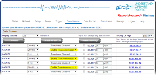
Visit the "Data stream" tab of the unit's web interface. Select "Enable Transform (reboot)" for all three streams, Z, N and E, from the instrument.
Click
 to reboot the digitiser and wait for the web page to reappear.
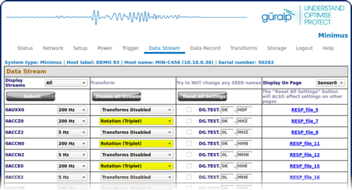
Visit the "Data stream" tab again and change the transform drop-down from "Pass-through" to "Rotation (triplet) for the Z stream from the instrument. The other two will change to match.
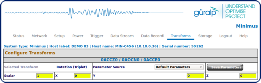
Move to the "Transforms" tab. Under "Configure Transforms", change the "Parameter Source" drop-down to "Saved User Parameters":
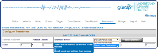
Populate the four boxes in the "Rotation (triplet)" section as follows:
Field | Value |
Scalar | cos(θ/2) |
X | 0 |
Y | 0 |
Z | sin(θ/2) |
90.6° ÷ 2 = 45.3°
sin(-45.3°) = 0.711
cos(-45.3°) = 0.703
where θ is the sign-reversed angle produced by Scream!.
For example: To configure the rotation of -90.6° as above, first negate the angle and then compute the sine and cosine of +90.6° ÷ 2, paying particular attention to the polarity (sign) of the answer:
and then populate the fields in the web page with:
Field | Value |
Scalar | 0.703 |
X | 0 |
Y | 0 |
Z | 0.711 |
Once the parameters have been entered, click
 in order to save the parameters to non-volatile memory. If you neglect to do this, the settings will revert to the defaults when the digitiser is next rebooted.
Collect some more data with the transformation active, and carry out another orientation calculation. The data from the down-hole instrument should now have a maximum coherence with the reference sensor at 0°. Check in particular that the sign of the rotation you have applied is correct.
as shown: