Chapter 5. Calculation Details
This section describes the concept of the strong motion calculations. The document SWA-RFC-STMN provides the details of the packet format.
5.1 Low Latency Waveform Data
Using the configuration given in section 3, the digitiser will transmit low latency data blocks. These are 20 sps blocks that are emitted every second. They can be turned off with the command 0 triggers and on with $77 triggers (or simply 7 triggers for a two-channel instrument).
Turning off the transmission of the blocks does not affect the strong motion calculations. The low latency streams are always computed, even if they are not transmitted or stored in flash, as they are used by the strong motion calculations to produce a strong motion data block.
The low latency data uses a different pre-decimation filter to the normal 20 sps data. You will see a difference between the two if they are turned on simultaneously. There are two differences between the normal and the low latency filter:
The low latency filter has a high-pass effect, with a corner frequency at approximately 0.001 Hertz (1000 seconds).
The low latency filter is implemented as an IIR (Infinite Impulse Response) rather than an FIR (Finite Impulse Response) filter. This implementation was chosen because an FIR filter requires many taps to produce a good cut-off, but more taps introduce more latency. An IIR filter can be implemented with far fewer taps, allowing the data to be retrieved in much shorter order.
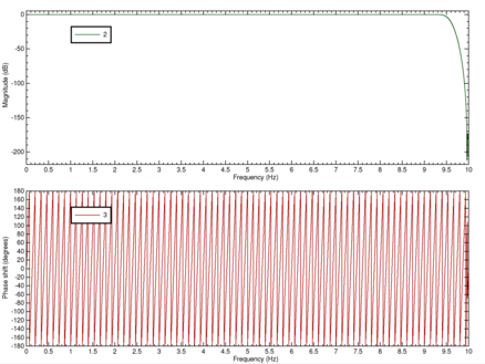
The low latency filter has a different phase and freqency response to the normal filter. Bode plots (filter response magnitude and phase plotted against frequency) for both types of filter are displayed below.
The Bode plots show the magnitude and phase shift of the response of each set of filters over a range of input frequencies. The normal pre-decimation filter (a cascaded divide by two and divide by five FIR filter) has a sharp cut-off point and rolls off very quickly. The low latency pre-decimation filter is a set of four cascaded first-order IIR filters. Its roll off is comparatively shallow and begins at a lower frequency.
The phase shift is actually a linear phase shift introduced by a pure time delay. The FIR filter used has a completely flat phase response, but is acausal. A pure time delay must be used so that the filter can be realised. This simply means that the output sample y(t) (where t is time) does not coincide with the input sample u(t) but instead to the sample u(t-n) for some constant n.
The bode plot for a normal 200 Hertz to 20 Hertz pre-decimation FIR filter looks like this:
while the low latency version looks like this:
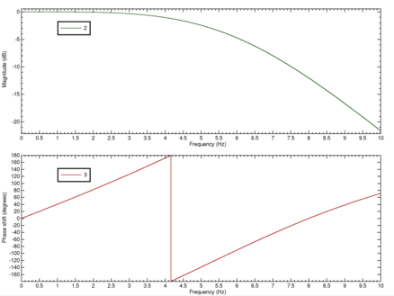
The high pass effect is present but cannot be seen on this scale.
5.2 Types of Strong Motion Result
The following strong motion results are calculated every second, in real-time. They are transmitted in the SM GCF block.
5.2.1 Windowed MMA (minimum, maximum and average)
The most basic strong motion result type is the minimum, maximum and average (arithmetic mean). This is computed every second and uses a 10 second sliding window (so the result at y(t) is based on input data from u(t) to u(t-10)).
This calculation finds the minimum, maximum and average number of counts, and then converts these numbers (in digital counts) into ground units using the calibration info in the info block. The result is in gal.
5.2.2 PGA (peak ground acceleration)
The peak ground acceleration is computed every second, and is the magnitude of the largest acceleration recorded in a 1s interval. The acceleration is simply the difference between the raw sampled value of the input and the sliding average from the windowed MMA data. The result is in gal.
5.2.3 RMS (root mean square)
The RMS is computed every second and is the root mean square of the digital counts for a one-second period. The DC offset of the signal is removed by subtracting the average from the MMA calculation. The RMS is a measure of the energy imparted to the digitiser during a one-second period. The result is in gal.
5.2.4 SI (spectral intensity)
The spectral intensity is a measurement that attempts to determine the amount of energy absorbed by structures in the vicinity of the sensor during an event. The calculation uses a series of frequency-dependent filters to model structures and performs an integration calculation to compute the expected velocity (pseudo-velocity) of these structures.
The result, in kine, is thus an indication of how fast a structure was moving and thus how likely it is to be damaged. SI corresponds very closely to physical damage.