MAN-040-0001 Güralp 40T User's Guide

Section Index: 5.1 The calibration pack 5.2 Calibration methods 5.3 Calibration with Scream! 5.4 Calibration with a hand‑held control unit

Chapter 5. Calibrating the 40T

5.1 The calibration pack

All Güralp sensors are fully calibrated before they leave the factory. Both absolute and relative calibration calculations are carried out. The results are given in the calibration pack supplied with each instrument:

Works Order : The Güralp factory order number including the instrument, used internally to file details of the sensor's manufacture.

Serial Number : The serial number of the instrument

Date : The date the instrument was tested at the factory.

Tested By : The name of the testing engineer.

There follows a table showing important calibration information for each component of the instrument, VERTICAL, NORTH/SOUTH, and EAST/WEST. Each row details:

Velocity Output (Differential) : The sensitivity of each component to velocity at 1 Hz, in volts per m/s. Because the 40T uses balanced differential outputs, the signal strength as measured between the +ve and –ve lines will be twice the true sensitivity of the instrument. To remind you of this, the sensitivities are given as 2 × (single-ended sensitivity) in each case.

Mass Position Output : The sensitivity of the mass position outputs to acceleration, in Volts per ms-². These outputs are single-ended and referenced to signal ground.

Feedback Coil Constant : A constant describing the characteristics of the feedback system. You will need this constant, given in Amperes per ms-², if you want to perform your own calibration calculations (see below.)

Power Consumption : The average power consumption of the sensor during testing, given in amperes and assuming a 12 Volt supply.

Calibration Resistor : The value of the resistor in the calibration circuit. You will need this value if you want to perform your own calibration calculations (see below.)

5.1.1 Poles and zeroes

Most users of seismometers find it convenient to consider the sensor as a “black box”, which produces an output signal V from a measured input x. So long as the relationship between V and x is known, the details of the internal mechanics and electronics can be disregarded.

This relationship, given in terms of the Laplace variable s, takes the form

In this equation

G is the acceleration output sensitivity (gain constant) of the instrument. This relates the actual output to the desired input over the flat portion of the frequency response.
A is a constant which is evaluated so that A × H (s) is dimensionless and has a value of 1 over the flat portion of the frequency response. In practice, it is possible to design a system transfer function with a very wide-range flat frequency response.
The normalising constant A is calculated at a normalising frequency value fm = 1 Hz, with s = j fm, where j = √–1.
H (s) is the transfer function of the sensor, which can be expressed in factored form:

In this equation Zi are the roots of the numerator polynomial, giving the zeros of the transfer function, and Pj are the roots of the denominator polynomial giving the poles of the transfer function.

In the calibration pack, G is the sensitivity given for each component on the first page, whilst the roots Zi and Pj, together with the normalising factor A, are given in the Poles and Zeros table. The poles and zeros given are measured directly at Güralp Systems' factory using a spectrum analyser. Transfer functions for the vertical and horizontal sensors may be provided separately.

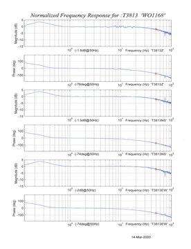
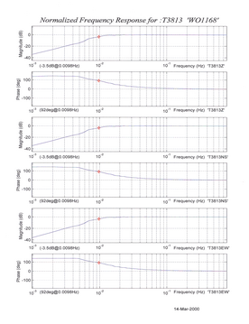
5.1.2 Frequency response curves

The frequency response of each component of the 40T is described in the normalised amplitude and phase plots provided. The response is measured at low and high frequencies in two separate experiments. Each plot marks the low-frequency and high-frequency cut-off values (also known as –3 dB or half-power points).

If you want to repeat the calibration to obtain more precise values at a frequency of interest, or to check that a sensor is still functioning correctly, you can inject calibration signals into the system using a Güralp digitiser or your own signal generator, and record the instrument's response.

5.1.3 Obtaining copies of the calibration pack

Our servers keep copies of all calibration data that we send out. In the event that the calibration information becomes separated from the instrument, you can obtain all the information using our free e-mail service. Simply e-mail caldoc@guralp.com with the serial number of the instrument in the subject line, e.g.

The server will reply with the calibration documentation in Word format. The body of your e-mail will be ignored.

Note: If you have a digital instrument, separate the serial numbers of the analogue part and the digital part with a space, as shown.

5.2 Calibration methods

Velocity sensors such as the 40T are not sensitive to constant DC levels, either as a result of their design or because of an interposed high-pass filter. Instead, three common calibration techniques are used.

Injecting a step current allows the system response to be determined in the time domain. The amplitude and phase response can then be calculated using a Fourier transform. Because the input signal has predominantly low-frequency components, this method generally gives poor results. However, it is simple enough to be performed daily.
Injecting a sinusoidal current of known amplitude and frequency allows the system response to be determined at a spot frequency. However, before the calibration measurement can be made the system must be allowed to reach a steady state; for low frequencies, this may take a long time. In addition, several measurements must be made to determine the response over the full frequency spectrum.
Injecting white noise into the calibration coil gives the response of the whole system, which can be measured using a spectrum analyser.

You can perform calibration either using a Güralp DM24 digitiser, which can generate step and sinusoidal calibration signals, or by feeding your own signals into the instrument through a hand-held control unit.

Before you can calibrate the instrument, its calibration relays need to be activated by pulling low the CAL ENABLE line on the instrument's connector for the component you wish to calibrate. Once enabled, a calibration signal provided across the CAL SIGNAL and SIGNAL GROUND lines will be routed through the feedback system. You can then measure the signal's equivalent velocity on the sensor's output lines. Güralp Hand-held Control Units provide a switch for activating the CAL ENABLE line.

5.3 Calibration with Scream!

Güralp digitisers provide calibration signal generators to help you set up your sensors. Calibration is most easily done through a PC running Güralp's Scream! software.

Depending on the digitiser type, sine-wave, step and broadband noise signal generators may be available. In this section, broadband noise calibration will be used to determine the complete sensor response in one action. Please refer to the digitiser's manual for information on other calibration methods.

In Scream!'s main window, right-click on the digitiser's icon and select Control.... Open the Calibration pane.
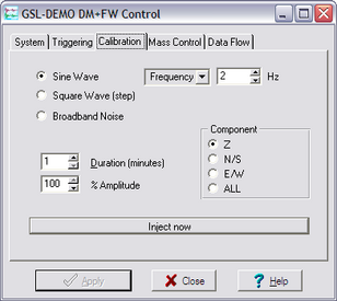
Select the calibration channel corresponding to the instrument, and choose Broadband Noise. Select the component you wish to calibrate, together with a suitable duration and amplitude, and click the button. A new data stream, ending Cn (n = 0 – 7) or MB, should appear in Scream!'s main window containing the returned calibration signal.
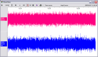
Open a WaveView window on the calibration signal and the returned streams by selecting them and double-clicking. The streams should display the calibration signal combined with the sensors' own measurements. If you cannot see the calibration signal, zoom into the WaveView using the scaling icons at the top left of the window or the cursor keys.
Drag the calibration stream Cn across the WaveView window, so that it is at the top.
If the returning signal is saturated, retry using a calibration signal with lower amplitude, until the entire curve is visible in the WaveView window.
If you need to scale one, but not another, of the traces, right-click on the trace and select Scale.... You can then type in a suitable scale factor for that trace.
Pause the WaveView window by clicking on the button.
Hold down and drag across the window to select the calibration signal and the returning component(s). Release the mouse button, keeping held down. A menu will pop up. Choose Broadband Noise Calibration.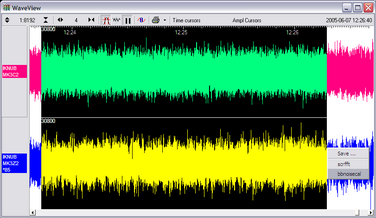
The script will ask you to fill in sensor calibration parameters for each component you have selected.

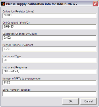
Most data can be found on the calibration sheet for your sensor. Under Instrument response, you should fill in the sensor response code for your sensor, according to the table below. Instrument Type should be set to the model number of the sensor.
If the file calvals.txt exists in the same directory as Scream!'s executable (scream.exe), Scream! will look there for suitable calibration values. A sample calvals.txt is supplied with Scream!, which you can edit to your requirements. Each stream has its own section in the file, headed by the line [instrument-id]. The instrument-id is the string which identifies the digitiser in the left-hand pane, e.g. GURALP-DEMO. It is always 6 characters (the system identifier) followed by a dash, then 4 characters (the serial number.)
For example:
[instrument-id]
Serial-Nos=T3X99
VPC=3.153,3.147,3.159
G=1010,1007,1002
COILCONST=0.02575,0.01778,0.01774
CALVPC=3.161
CALRES=51000
TYPE=sensor-type
RESPONSE=response-code
Click . The script will return with a graph showing the response of the sensor in terms of amplitude and phase plots for each component (if appropriate.)
The accuracy of the results depends on the amount of data you have selected, and its sample rate. To obtain good-quality results at low frequency, it will save computation time to use data collected at a lower sample rate; although the same information is present in higher-rate streams, they also include a large amount of high-frequency data which may not be relevant to your purposes.

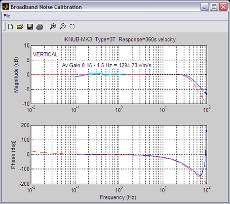
The bbnoisecal script automatically performs appropriate averaging to reduce the effects of aliasing and cultural noise.

5.3.1 Sensor response codes

Sensor	Sensor type code	Units (V/A)
40T-1 or 6T-1, 1 s – 50 Hz response	CMG-40_1HZ_50HZ	V
40T-1 or 6T-1, 1 s – 100 Hz response	CMG-40_1S_100HZ	V
40T-1 or 6T-1, 2 s – 100 Hz response	CMG-40_2S_100HZ	V
40T-1 or 6T-1, 10 s – 100 Hz response	CMG-40_10S_100HZ	V
40, 20 s – 50 Hz response	CMG-40_20S_50HZ	V
40, 30 s – 50 Hz response	CMG-40_30S_50HZ	V
40, 60 s – 50 Hz response	CMG-40_60S_50HZ	V

5.4 Calibration with a hand-held control unit

If you prefer, you can inject your own calibration signals into the system through a hand-held control unit. The unit includes a switch which activates the calibration relay in the seismometer, and 4 mm banana sockets for an external signal source. As above, the equivalent input velocity for a sinusoidal calibration signal is given by

where V is the peak-to-peak voltage of the calibration signal, f is the signal frequency, R is the magnitude of the calibration resistor and K is the feedback coil constant. R and K are both given on the calibration sheet supplied with the 40T.

The calibration resistor is placed in series with the transducer. Depending on the calibration signal source, and the sensitivity of your recording equipment, you may need to increase R by adding further resistors to the circuit.