Chapter 4. Calibrating Güralp 5U sensors

The 5U accelerometer is supplied with a comprehensive calibration document, and it should not normally be necessary to calibrate it yourself. However, you may need to check that the response and output signal levels of the sensor are consistent with the values given in the calibration document.

4.1 Principle of operation

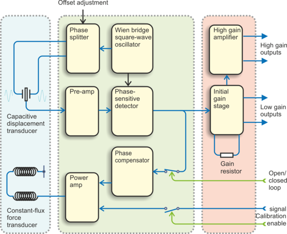
The 5U is a force-feedback instrument. An inertial mass with a pendulum suspension forms the centre pole of a centre-tapped, variable capacitor, energised with anti-phase sine-waves. The signal from the mass is fed into a feedback loop which drives an electromagnetic coil attached to the mass, such that the mass is maintained centrally in the gap. The current required to do so it proportional to the acceleration experienced by the instrument. The basic arrangement is shown below.

4.2 Absolute calibration

The sensor's response (in V/ms-2) is measured at the production stage by tilting the sensor through 90 ° and measuring the acceleration due to gravity. The local value of g at the Güralp Systems production facility is known to an accuracy of five digits.

4.3 Relative calibration

In addition to the response of the sensor, several other variables are calibrated at the production stage. Using these values, you can convert directly from counts (as measured in Scream!) to acceleration values and back. You can check any of these values by performing calibration experiments.

Güralp sensors and digitisers are calibrated as follows:

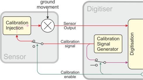
In this diagram a Güralp digitiser is being used to activate the calibration enable line and to inject a calibration signal into the sensor. The signal can be a sine wave, a step function or broadband noise, depending on your requirements. As well as going into the sensor, the calibration signal is returned to the digitiser on the dedicated calibration input channel. The calibration signals and sensor output all travel down the same cable from the sensor to an analogue input port on the digitiser.

The signal injected into the sensor gives rise to an equivalent acceleration (marked “EA” on the above diagram) which is added to the measured acceleration to provide the sensor output. Because the injection circuitry, when disconnected) can be a source of noise, a “Calibration enable” line from the digitiser is provided which can disconnect the calibration circuit when it is not required. Depending on the factory settings, the Calibration enable line must be either provided with a DC voltage source (+5 to +10 V) or held low during calibration: this is given on the sensor's calibration sheet.

The equivalent acceleration corresponding to 1 V of signal at the calibration input is measured at the factory, and can be found on the 5U calibration sheet. The calibration sheet for the digitiser documents the number of counts corresponding to 1 V of signal at each input. The sensor transmits the signal differentially, over two separate lines, and the digitiser subtracts one from the other to improve the signal-to-noise ratio by increasing common mode rejection. As a result of this, the sensor output should be halved to give the true acceleration.

All sensors are tuned at the factory to produce 1 V of output for 1 V input on the calibration channel. For example, a sensor with an acceleration response of 0.25 V/ms-2 should produce 1 V output given a 1 V calibration signal, corresponding to 1/0.25 = 4 V/ms-2 = 0.408 g of equivalent acceleration.

The following section explains how to calibrate Güralp 5U sensors using a DM24 series digitiser and a computer running Güralp Systems Scream! Software.

4.4 Using a DM24 series digitiser for calibration

This section describes how to perform a broadband noise calibration. For other calibration techniques, please see our web site, http://www.guralp.com/.

4.4.1 The calibration process

• In Scream!'s main window, right-click on the digitiser's icon and select Control.... In the resulting dialogue, open the Calibration tab.

  

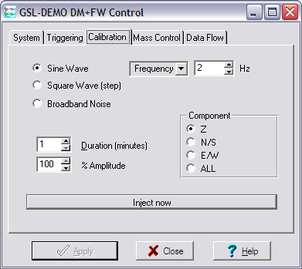
• Choose “Broadband Noise” as the calibration type. In the “Component” frame, select the channel corresponding to the instrument (typically Z for single-instrument set-ups). Set the amplitude to 100% and select a suitable duration (at least ten times the longest period in which you are interested), then click Inject now. A new stream ending Cn (where n represents the tap identification number) should appear in Scream!'s main window containing the returned calibration signal.

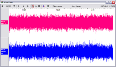
• Open a WaveView window on the calibration signal and the returned streams by selecting them and double-clicking. The streams should display the calibration signal combined with the sensors' own measurements. If you cannot see the calibration signal, zoom into the WaveView using the scaling icons at the top left of the window or the cursor keys.

  

• If you need to scale one, but not another, of the traces, right-click on the trace and select Scale.... You can then type in a suitable scale factor for that trace.

• Pause the Waveview window by clicking on the icon.

• Hold down the shift key () and drag across the window to select the calibration signal and the returning component(s). Release the mouse button, keeping held down. A context menu will pop up: choose “Broadband Noise Calibration”.

• The script will ask you to fill in sensor calibration parameters for each component you have selected.

  

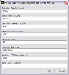
  Most data can be found on the calibration sheet for your sensor. The fields in this form are described in detail in section 4.4.2.

• Click . The script will return with a graph showing the response of the sensor in terms of amplitude and phase, plotted against frequency. The accuracy of the results depends on the amount of data you have selected and its sample rate. To obtain good-quality results at low frequency, it will save computation time to use data collected at a lower sample rate; although the same information is present in higher-rate streams, they also include a large amount of high-frequency data which may not be relevant to your purposes.

  

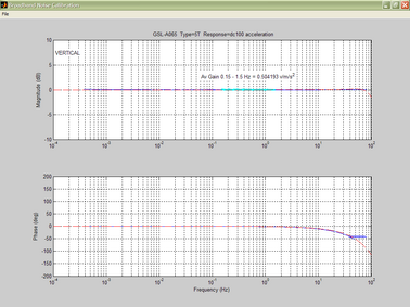
  The noise calibration script automatically performs appropriate averaging to reduce the effects of aliasing and cultural noise.

4.4.2 Calibration values

The calibration parameters required by the script are as follows:

• Calibration Resistor (ohms) : The value of the calibration resistor, in Ω, as given on the sensor calibration sheet. This is normally 1 Ω for Güralp 5U instruments.

• Coil Constant (A/m s⁻²) : The coil constant for the component being calibrated, in Amps per ms-2, as given on the sensor calibration sheet.

• Calibration Channel µV/Count : The sensitivity of the digitiser’s calibration channel, in μV per count, as given on the digitiser calibration sheet.

• Sensor Channel µV/Count : The sensitivity of the digitiser’s input channel, in μV per count, as given on the digitiser calibration sheet.

• Instrument Type : The model number of the instrument or any other desired text to be displayed in the title of the output graph.

• Instrument Response : The theoretical response of the instrument, as defined by its poles and zeroes. This information is used to generate a theoretical response curve.

  The response is entered as a code, as shown in the following table:

• FFT window size : This value specifies the FFT length used in the calculation and, hence, the frequencies at which calibration is performed. The default value is automatically chosen to give optimal results, and you should not normally need to change it.

• Serial Number (optional) : A serial number to be displayed in the title of the graph.

4.4.3 Calibration using non-Güralp equipment

If you prefer, you can inject your own signals into the system at any point (together with a Calibration enable signal, if required) to provide independent measurements, and to check that the voltages around the calibration loop are consistent. For reference, a DM24-series digitiser will generate a calibration signal of around 16000 counts / 4 V when set to 100% (sine-wave or step), and around 10000 counts / 2.5 V when set to 50%.