Chapter 3. Examples
3.1 Conventions
The following examples assume that we have incoming live data from a digitiser with System ID “DEMO” and Serial Number "INP". The digitiser is producing three streams “INPZ2, “INPN2” and “INPE2” for the vertical, North/South and East/West components, respectively.
Note: Although the examples below span multiple lines for legibility, recall that they must be entered on a single line in the expressions section of scream.ini.
3.2 Recipes
3.2.1 Gain
To increase the gain of a stream, use simple multiplication. The expression:
DEMO_OUTZ2 = STREAM_DEMO_INPZ2 * 2 // Doubled
produces a new output stream with amplitude of twice the input, while
DEMO_OUTZ2 = STREAM_DEMO_INPZ2 * 1.02 // +2%
produces a new output stream with a 2% increase in gain.
In both cases, the new output stream will have System ID DEMO and Stream ID OUTZ2. The Instrument, as displayed in Scream's source tree, will be "Doubled" in the first case and "+2%" in the second.
3.2.2 Resultant
The expression
DEMO_OUT3D = SquareRoot( SumOfSquares(
STREAM_DEMO_INPZ2, STREAM_DEMO_INPN2, STREAM_DEMO_INPE2
) ) // DEMO3D
computes a three-dimensional resultant. A two-dimensional (horizontal) resultant can be computed with
DEMO_OUT2D = SquareRoot( SumOfSquares(
STREAM_DEMO_INPN2, STREAM_DEMO_INPE2
) ) // DEMO2D
Note that the SquareRoot() and SumOfSquares() functions are computationally cheaper than the equivalent "long-hand" expressions involving ^0.5 and ^2.
3.2.3 Time-shift
To introduce a one-sample offset into a data-stream, use the following expression:
DEMO_OUTZ2 = STREAM_DEMO_INPZ2[-1] // DELAYED
A negative index refers to samples in the past, whilst a positive index refers to samples in the future. Only samples in Scream's stream buffer can be accessed so, for large time offsets, you may need to increase the maximum stream buffer size. Please see the Scream manual, MAN-SWA-0001 for details.
Any offset which can be represented by a 32-bit number can be used but please note that where negative offsets are used, sufficient data must be accumulated before the output can start and, where positive offsets are used, a delay must be imposed on the output.
3.2.4 Differentiation
By using temporal subscripting, complex operations can be easily implemented. Differentiation of the input signal is simply a case of subtracting the previous sample from the current sample (taking the difference), then multiplying by the sample rate.
The following expression converts the input velocity stream to an output acceleration stream:
DEMO_OUTZ2 = ( STREAM_DEMO_INPZ2 – STREAM_DEMO_INPZ2[-1] )
* STREAMSPS // ACCEL
Note the use of the STREAMSPS token, which will be set to the sample rate of the output data stream. See section 2.3.2.4 for more information about using tokens.
3.2.5 Filtering
There are many techniques which can be used to implement digital filters and a discussion of these is beyond the scope of this document. A simple high-pass filter, however, can be implemented with an expression such as:
DEMO_OUTZ2 = 0.999372076005564 * ( STREAM_DEMO_OUTZ2[-1] +
STREAM_ DEMO_INPZ2 - STREAM_DEMO_INPZ2[-1] ) // HPF
The constant value, α, (0.999372076005564 in this example) determines the corner frequency of the filter and can be calculated from:

where p is the sample period in seconds (the reciprocal of the sample rate in Hertz) and fc is the desired corner frequency in Hertz.
3.2.6 Rotation
This example uses the functions ROTATEX() and ROTATEY(), which were described in section 2.3.2.4. The two are normally used together.
The following expressions generate N/S and E/W streams which are rotated 32 degrees from the corresponding input streams:
DEMO_OUTN2 = ROTATEX( STREAM_DEMO_INPN2, STREAM_DEMO_INPE2, 32 ) // ROTATED
DEMO_OUTE2 = ROTATEY( STREAM_DEMO_INPN2, STREAM_DEMO_INPE2, 32 ) // ROTATED
The two streams will appear together in Scream's source tree under theinstrument name "ROTATED".
3.2.7 Integration (broken!)
Integration can be usefully simulated using the trapezoidal rule. Geometrically, this approximates the traditional "area under the curve" with a series of trapezoids:
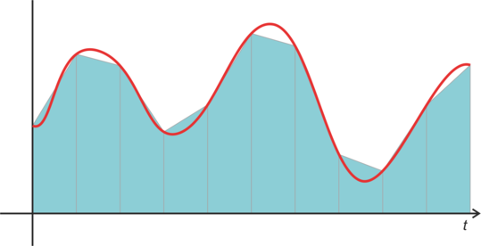
In the example above, the integral of the red curve is approximated by the sum of the areas of the blue trapezoids.
This is particularly convenient with sampled data because the width of each trapezoid can be set to be the sample period, so the area under each trapezoid can be calculated easily from the period and the values of two adjacent samples.
The following expression integrates a velocity stream to produce a displacement stream:
DEMO_OUTZ2 = STREAM_DEMO_OUTZ2[-1] +
( STREAM_DEMO_INPZ2 + STREAM_DEMO_INPZ2[-1] )
/ ( STREAMSPS * 2 ) // DISP
Note that the right-hand side of the expression includes a past sample from the virtual stream being generated.
Note: The result of a naive integration like this will over-flow (or under-flow) as the underlying mathematical integral tends towards ±∞. This can be avoided by applying a high-pass filter to the original data and integrating the result in a two-stage process, as described in the following section.
3.2.8 Chained expressions: High-pass filter + Integration
The previous recipe is unusable because any offset in the input stream will result in the output moving to the upper or lower extreme as the underlying integral tends towards infinity. The solution is to apply a high-pass filter to the input data and then derive the integral from the filtered data, rather than from the raw velocity data. This involves chaining two expressions together so that the output of one is the input of the next. This can be achieved using the following syntax:
DEMO_HPFZ2 = 0.999372076005564 * ( STREAM_DEMO_HPFZ2[-1] +
STREAM_ DEMO_INPZ2 - STREAM_DEMO_INPZ2[-1] ) // HPF
DEMO_OUTZ2 = STREAM_DEMO_OUTZ2[-1] +
( STREAM_DEMO_HPFZ2 + STREAM_DEMO_HPFZ2[-1] )
/ ( STREAMSPS * 2 ) // DISP
The first expression high-pass filters the data from DEMO_INPZ2 to create a virtual stream DEMO_HPFZ2. The second expression integrates the result to produce the output stream DEMO_OUTZ2.