Chapter 3. The procedure

The temperature training has four parts: preparation, execution, finalisation and testing. Each is covered below.

3.1 Preparation

These steps should be carried out first.

Place the Fortimus in a location where you can expect the temperature to vary slowly but considerably during the training. It needs to be exposed to a range of temperatures wider than that expected in the final operating environment to ensure that the look-up-table is sufficiently populated. Once placed, allow it to acclimatise.

Note: Avoid placing the unit in direct sunlight because this is likely to cause the temperature to change too rapidly.
Use Discovery to update the Fortimus to the latest stable firmware (at least 2.1-17622). This will reboot the system.
Attach a GNSS receiver and wait for the GNSS to lock. Check the stability using the Status tab of the Fortimus webpage.

Note: The GNSS takes approximately fifteen minutes to lock
On the Data stream tab of the Fortimus webpage , enable the channels 0TMPA0, 0CVDAC, 0CGPSO and 0CPLLDAC for data streaming at 10 Hz.

Note: Unless all of these channels were previously enabled, you will need to reboot the Fortimus after enabling them all.
Open Discovery, double click your Fortimus and select Console.
The temperature-training lookup-table is a system resource called nand_lut 1. Enter the command
resource show
and check the output to see if the resource nand_lut 1 exists. If it does not, enter the command
resource add nand_lut 1
reboot

Note: If you have just had to reboot, wait until the system has booted fully and then access the console again.
In normal use, the Fortimus will be continually consulting the lookup table, preventing writing.. To stop this, enter the command
lut run 0
Put the Fortimus into training mode by entering the command
lut train 1
in the console

This completes the preparatory steps.

3.2 Training

The Fortimus, as it is now configured, will train itself while the ambient temperature varies. It should be exposed to a range of temperatures wider than that expected in the final operating environment so that the look-up-table is sufficiently populated. This typically requires running overnight at least once.

Note: The longer that you can leave the Fortimus in training mode, the more accurate the results will be. This is because the offset associated with each temperature is the average of the calculated offsets; the more offsets collected at each temperature, the more accurate this average is likely to be.

To monitor the progress of the training:

Go to the Live View window in Discovery and select a period of your data
Right-click and, from the pop-up context menu, select decimation → Clock LUT. This will show the plotted temperature data

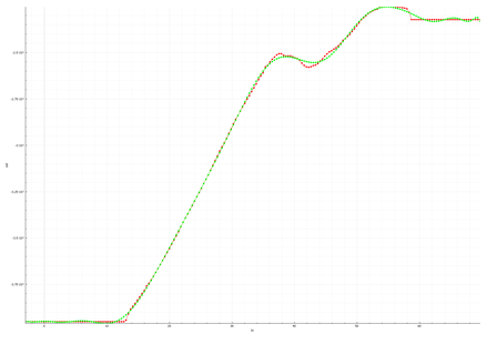
Note: The plot shows two lines: one red and one green. The red line is the absolute temperature value at a given point, and the green is the smoothed rolling average. The curve will look linear to begin with as the temperature slowly ramps up and then forms a distorted S shape, as shown in the example.
You can check the populated temperature training table by entering
lut show
in the Fortimus console. The format of this output is shown in chapter 4. Training is complete when the chosen range of temperatures (third column - in millidegrees C) is fully covered by the table.

3.3 Finalisation

Once you have gather sufficient training data

Stop the training by entering
lut train 0
in the Fortimus console.
If the table is incomplete, it can be extended by using the command
lut extend
to fill the table by a combination of interpolation and extrapolation.

Note: If the table is already full then this command will not do anything
Enter the command
lut save
to save the table to non-volatile storage
Re-start the clock lookup function by entering
lut run 1

This completes the finalisation.

Note: If you wish to re-train the system, execute lut clear followed by

lut run 0

lut train 1

then re-start the instructions from section 3.2.

3.4 Testing

Once the training is complete, we recommend performing a time drift test by setting up two Fortimus units next to each other. We will synchronise both and then allow the unit we have trained to drift for 24 hours before comparing the sample clocks using a common marker found in the data.

Ensure that the configuration of both instruments is identical.

Note: Higher sample rates will give more accurate results.
Let both instruments synchronise their sample clocks to the GNSS and allow the temperature to stabilise
Disconnect the GNSS receiver from the unit which you have just trained
Allow both instruments to continue running for around 24 hours.
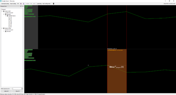
From Discovery, open a Live View window containing the acceleration streams and select a significant signal spike across two seismic channels: one for each Fortimus.
Zoom into the selected period of data and compare the arrival times of the signal for each instrument, as shown in the example below:

If you are satisfied with the synchronicity between the two instruments, the test is complete.