Chapter 4. Calibrating the CD24

4.1 Calibration methods

Sensors attached to the CD24 can be calibrated using the built-in signal generator. There are three common calibration techniques used.

• Injecting a step current allows the system response to be determined in the time domain. The amplitude and phase response can then be calculated using a Fourier transform. Because the input signal has predominantly low-frequency components, this method generally gives poor results. However, it is simple enough to be performed daily.

• Injecting a sinusoidal current of known amplitude and frequency allows the system response to be determined at a spot frequency. However, before the calibration measurement can be made the system must be allowed to reach a steady state; for low frequencies, this may take a long time. In addition, several measurements must be made to determine the response over the full frequency spectrum.

• Injecting white noise into the calibration coil gives the response of the whole system, which can be measured using a spectrum analyser.

Further information about calibration is available on the Güralp Systems Web site.

4.2 Noise calibration with Scream!

A connected instrument can be calibrated using the digitiser's pseudo-random broadband noise generator, along with Scream!'s noise calibration extension. The extension is part of the standard distribution of Scream! and contains all the algorithms needed to determine the complete sensor response in a single experiment.

• In Scream!'s main window, right-click on the digitiser's icon and select Control.... Open the Calibration pane.

• Select the calibration channel corresponding to the instrument, and choose Broadband Noise. Select the component you wish to calibrate, together with a suitable duration and amplitude, and click Inject now. A new data stream ending Cn (n = 0 – 7) should appear in Scream!'s main window containing the returned calibration signal.

  

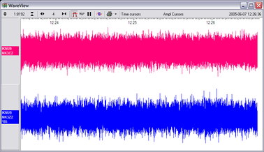
• Open a Waveview window on the calibration signal and the returned streams by selecting them and double-clicking. The streams should display the calibration signal combined with the sensors' own measurements. If you cannot see the calibration signal, zoom into the Waveview using the scaling icons at the top left of the window or the cursor keys.

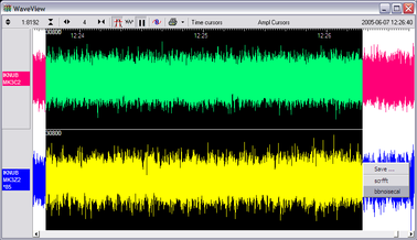
• Drag the calibration stream Cn across the Waveview window, so that it is at the top.

• If the returning signal is saturated, retry using a calibration signal with lower amplitude, until the entire curve is visible in the Waveview window.

• If you need to scale one, but not another, of the traces, right-click on the trace and select Scale.... You can then type in a suitable scale factor for that trace.

• Pause the Waveview window by clicking on the icon.

• Hold down SHIFT and drag across the window to select the calibration signal and the returning component(s). Release the mouse button, keeping SHIFT held down. A menu will pop up. If it doesn't it is likely because you have not selected at least two signals (calibration and the returning components)

• Choose Broadband Noise Calibration.

  

• The script will ask you to fill in sensor calibration parameters for each component you have selected.

  

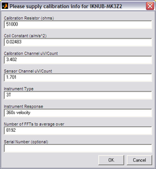
  Most data can be found on the calibration sheet for your sensor. Under Instrument response, you should fill in the sensor response code for your sensor, according to the table below. Instrument Type should be set to the model number of the sensor.

  If the file calvals.txt exists in the same directory as Scream!'s executable (scream.exe), Scream! will look there for suitable calibration values.

  See the Scream! manual for full details of this file. Alternatively, you can edit the sample calvals.txt file supplied with Scream!.

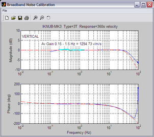
• Click OK. The script will return with a graph showing the responsivity of the sensor in terms of amplitude and phase plots for each component (if appropriate.)

  The accuracy of the results depends on the amount of data you have selected, and the sample rate. To obtain good-quality results at low frequency, it will save computation time to use data collected at a lower sample rate; although the same information is present in higher-rate streams, they also include a large amount of high-frequency data which may not be relevant to your purposes.

  

  The calibration script automatically performs appropriate averaging to reduce the effects of aliasing and cultural noise.

4.2.1 Sensor response codes