Chapter 4. Calibration

The 5T is supplied with a comprehensive calibration document, and it should not normally be necessary to calibrate it yourself. However, you may need to check that the response and output signal levels of the sensor are consistent with the values given in the calibration document.

4.1 Absolute calibration

The sensor's response (in V/ms-2) is measured at the production stage by tilting the sensor through 90 ° and measuring the acceleration due to gravity. Local g at the Güralp Systems production facility is known to an accuracy of 5 digits. In addition, sensors are subjected to the “wagon wheel” test, where they are slowly rotated about a vertical axis.

The response of the sensor traces out a sinusoid over time, which is calibrated at the factory to range smoothly from 1g to –1g without clipping.

4.2 Relative calibration

The response of the sensor, together with several other variables, is measured at the factory. The values obtained are documented on the sensor's calibration sheet. Using these, you can convert directly from voltage (or counts as measured in Scream!) to acceleration values and back. You can check any of these values by performing calibration experiments.

Güralp sensors and digitizers are calibrated as described below.

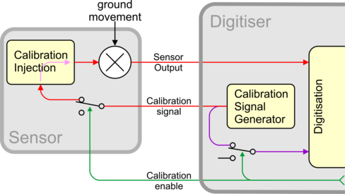
In this diagram a Güralp digitizer is being used to inject a calibration signal into the sensor. This can be either a sine wave, a step function or broad-band noise, depending on your requirements. As well as going to the sensor, the calibration signal is returned to the digitizer on a full rate channel (older digitizers used one of the 4 Hz auxiliary (Mux) channels). The calibration signals and sensor output all travel down the same cable from the sensor to an analogue input port on the digitizer.

The signal injected into the sensor gives rise to an equivalent acceleration (EA on the above diagram) which is added to the measured acceleration to provide the sensor output. Because the injection circuitry can be a source of noise, a Calibration enable line from the digitizer is provided which disconnects the calibration circuit when it is not required. Depending on the factory settings, the Calibration enable line must be either allowed to float high (+5 to +10 V) or held low (0V, signal ground) during calibration: this is specified on the sensor's calibration sheet.

The equivalent acceleration corresponding to 1 V of signal at the calibration input is measured at the factory, and can be found on the sensor calibration sheet. The calibration sheet for the digitizer documents the number of counts corresponding to 1 V of signal at each input port.

The sensor transmits the signal differentially, over two separate lines, and the digitizer subtracts one from the other to improve the signal-to-noise ratio by increasing common mode rejection. As a result of this, the sensor output should be halved to give the true acceleration.

CMG-5T instruments are tuned at the factory to produce 1 V of output for 1 V input on the calibration channel. For example, a sensor with an acceleration response of 0.25 V/ms-2 should produce 1 V output given a 1 V calibration signal, corresponding to 1/0.25 = 4 ms-2 = 0.408 g of equivalent acceleration.

4.3 Calibrating accelerometers

Both the DM24 digitizer and Scream! software allow direct configuration and control of any attached Güralp instruments. For full information on how to use a DM24 series digitizer, please see its own documentation. If you are using a third-party digitizer, you can still calibrate the instrument as long as you activate the Calibration enable line correctly and supply the correct voltages.

• In Scream!'s main window, right-click on the digitizer's icon and select Control.... Open the Calibration pane.

• Select the calibration channel corresponding to the instrument, make any other choices you require, and click Inject now. A new data stream, ending Cn (n = 0 – 7) or MB, should appear in Scream!'s main window containing the returned calibration signal.

• Open a WaveView window on the calibration signal and the returned streams by selecting them and double-clicking. The streams should display the calibration signal combined with the sensors' own measurements. If you cannot see the calibration signal, zoom into the WaveView using the scaling icons at the top left of the window or the cursor keys.

• If you need to scale only one of the traces, right-click on the trace and select Scale.... You can then type in a suitable scale factor for that trace.

• Click on Ampl Cursors in the top right hand corner of the window. A white square will appear inside the WaveView at the top left. This is in fact two superimposed cursors.

• Drag one cursor down to be level with the lowest point of the signal trace.

• Drag the other down to be level with the highest point. In the following example, a step function of 1 minute duration has been applied to the Z3 stream. Note that ground movements continue to be observed, superimposed on the returning calibration signal.

  

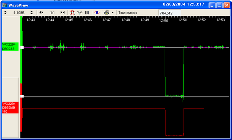
  The Ampl Cursors button will now be displaying a value, which is the strength of the returning signal in counts (doubled, if using a sine wave). Measure the other two signal strengths in this manner.

  Note that if you have used the Scale... option described above, you will need to take the scale factor into account to produce the correct number of counts. In the example, the MB (calibration input) signal has been scaled by a factor of 40, so the signal strength as measured by the Ampl Cursors must be divided by 40 to yield the correct value.

• Convert to volts using the µV/Bit values given on the digitizer's calibration sheet for the various input ports, and compare the returned signal with the input calibration signal (MB).

• In the example, the following data are now known:

The calibration sheets provide us with the remaining values needed to calibrate the sensor:

From these we calculate that the calibration signal is producing 697,221 × 3.491621 = 2,434,431 µV (2.434 V). This corresponds to an equivalent input acceleration of 2.434 × 1.968 = 4.791 ms-2.

The sensor's acceleration response is given as 0.254 V/ms-2, so that an acceleration of 4.791 ms-2 will produce an output of 0.254 × 4.791 = 1.217 V (1,216,904 µV), which corresponds to a count number at the digitizer's input port of
1,216,904 / 3. 507212 = 346,972 counts.

Because this calibration is being carried out with a differential-output sensor, the count number observed at the digitizer should be double this: 693,944 counts. All Güralp Systems sensors use balanced differential outputs.

The actual signal at the digitizer of 701,512 counts is within 1.5% of this value, indicating that the sensor is adequately calibrated.

• If you know the local value of g, you can also perform absolute calibration by tilting the sensor by 90 ° and varying the calibration signal until it precisely compensates for the signal generated due to gravity.

• Calibrate any other sensors connected to the digitizer in the same way. You must wait for the previous calibration to finish before doing this: clicking Inject now has no effect whilst the Calibration enable relay is open.

If you prefer, you can inject your own signals into the system at any point (together with a Calibration enable signal, if required) to provide independent measurements, and to check that the voltages around the calibration loop are consistent. For reference, a DM24-series digitizer will generate a calibration signal of around 16000 counts / 4 V when set to 100% (sine-wave or step), and around 10000 counts / 2.5 V when set to 50%.