Chapter 4. Getting started
4.1 System set-up
Güralp highly recommends exploring and gaining familiarity with the Minimus inside your lab before installation in an outdoors environment.
A typical set-up for the Minimus connected to an analogue sensor (including an optional digital Radian Post-hole instrument) is shown in the figure below:
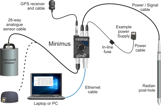
To get started, connect the cables as shown in the figure above and as described in section 3.2 (and, optionally, Section 4.3 of the Radian manual, MAN-RAD-0001).
Power up the Minimus using a power supply with a DC output of between 10 and 36 Volts. We recommend fitting an in-line 3.5 A anti-surge fuse in the positive power lead to protect the external wiring of the installation. The Minimus will, in turn, provide power to all connected instruments.
Caution: Observe the correct polarity when connecting the power supply. The red lead (from pin B) must be connected to the positive terminal, typically labelled “+”, and the black lead (from pin A) must be connected to the negative terminal, typically labelled “-”. An incorrect connection risks destroying the digitiser, the power supply and any connected instruments.
If the Minimus is directly connected to a laptop or PC using the blue Ethernet cable, make sure that the laptop or PC is configured to obtain an I.P. address automatically. More details on how to correctly configure the connection using APIPA (Automatic Private I.P. Addressing) are in section 13.
4.2 Güralp Discovery software installation
To view live waveforms, and to control and configure the Minimus and connected sensors, you will need to use Güralp Discovery software.
Visit www.guralp.com/sw/download-discovery.shtml for links for all available platforms (currently Windows 32-bit and 64-bit, macOS 64-bit and Linux 64-bit).
Download the installer appropriate for your architecture and operating system, run the installer and follow the instructions on screen. (Full details of installation and upgrading are in section 12.)
Note: Windows users may have to reconfigure the Windows FireWall in order to allow Discovery to communicate properly. Please see section 12.4 for full details. Brief instructions are below.
Under Windows, the first time that you start Discovery, Windows may ask you to specify how you wish Discovery to interact with the Windows Firewall. Because Discovery requires network communication in order to function, it is important that you understand the options available.
The following screen is displayed:
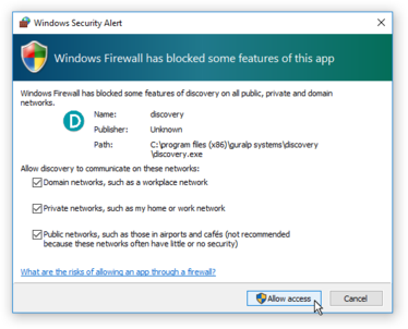
The screen provides three check-boxes which indicate whether Discovery can communicate with networked devices in the “Domain” profile, the “Private” profile or the “Public” profile. (Profiles are also known as “network locations”.)
The “Domain” profile applies to networks where the host system can authenticate to a domain controller. The “Private” profile is a user-assigned profile and is used to designate private or home networks. The default profile is the “Public” profile, which is used to designate public networks such as Wi-Fi hotspots at coffee shops, airports, and other locations.
For a more complete discussion of this topic, please see www.tenforums.com/tutorials/6815-network-location-set-private-public-windows-10-a.html or your Windows documentation.
Once you have specified your firewall preferences, Discovery displays a main window which normally shows a list of both locally and remotely connected instruments. If you close this main window, Discovery will quit.
Discovery will initially “listen” for connected instruments on your local network. This mode can be refreshed by clicking the  button or by pressing the short-cut keys
  +
+ . These features are identified below:
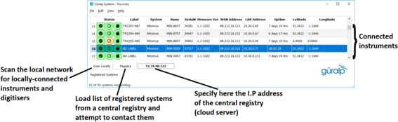
You can add instruments to the list by right-clicking in the blank area and selecting "Add device" or choosing this option from the Edit menu:
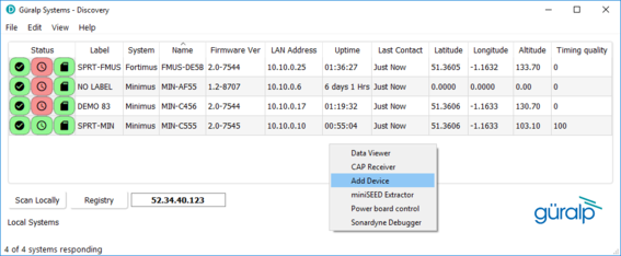
The following dialogue is displayed:
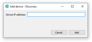
Enter the I.P. address of the Minimus (or other device, such as Güralp Affinity) to be added and click the  button. The newly added device will appear in the device list.
Note: The newly added device will be removed from the list and not automatically re-added if a local network scan is performed.
You can choose which information is shown for each device in the main window. You can select which columns to display – and hide unwanted ones – by clicking on "Show” from the "View" menu.
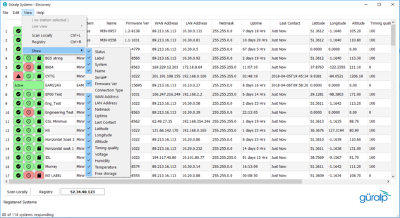
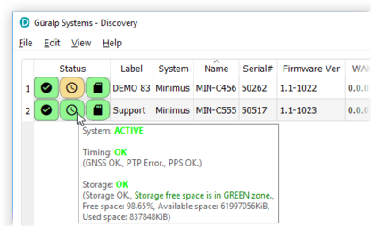
The “Status” column is composed of three icons that represent the Minimus connectivity status (whether Minimus is reachable/active or not), timing status (GNSS or PTP) and storage status (primary/secondary) respectively.
Hovering the mouse over any of these three icons will display tool-tips giving a brief description of the status including, for the timing indicator, details of which timing subsystems are operating:
Within Discovery, internal and connected sensors are referred to as follows:
Sensor | Minimus designation | ⨹ Minimus+ designation |
All internal sensors | Sensor 0 | Sensor 0 |
First analogue sensor | Sensor 0 | Sensor 0 |
⨹ Second analogue sensor | n/a | Sensor 1 |
First Radian (digital sensor) | Sensor 1 | Sensor 2 |
Second Radian (digital sensor) | Sensor 2 | Sensor 3 |
Third Radian (digital sensor) | Sensor 3 | Sensor 4 |
… | … | … |
Last Radian (digital sensor) | Sensor 8 | Sensor 8 |
4.3 Viewing waveforms and system state-of-health
Waveform data recorded by the Minimus’ internal sensors and other connected sensors can be viewed using several methods, which are described in the following sections.
4.3.1 Using Discovery’s “Live View” window
4.3.1.1 Main features
Discovery offers a versatile live waveform/data viewer. To open the Viewer, in Discovery’s main window, select an instrument and, from the View tab in the toolbar, select “Live View”.
The menu will then present three options for data streaming:
GDI and GCF channels
GDI only
GCF only
The GCF option uses the Scream! Protocol to stream data in GCF packets of, typically, 250, 500 or 1,000 samples. The GDI protocol streams data sample-by-sample and also allows the sending of each instrument's calibration parameters so that data can be expressed in terms of physical units rather than digitiser counts.
Güralp recommends using the “GDI only” option for waveform viewing.
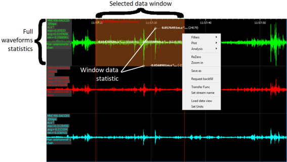
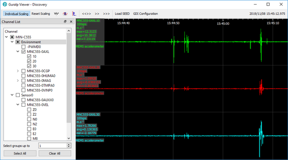
The main features of – and the key buttons within – the Live View window are shown in the following screen-shot. Basic amplitude and time zoom functions are given in the Window zoom controls panel and streams can be easily added to or removed from the window by using the check-boxes in the left panel.
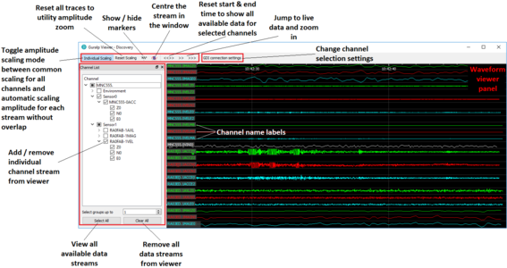
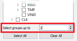
The channels are divided in groups with different hierarchical importance. The most important are the velocity/acceleration channels with higher sample rates: these belong to group 1. The least important belong to group 6, which includes humidity, temperature, clock diagnostics etc. When the live view is launched, only the channels in group 1 are selected. It is possible to change this setting by selecting a different group number from the “Select group up to” box at the bottom of the channel list.
When only few channels are selected for viewing, the channel name labels also show data statistics, including the maximum, minimum and average amplitudes in physical units.
If too many channels are in view for this information to be visible, you can left-click on a label and the label and trace will then expand to half the height of the screen, revealing these statistics. The other channels will be compressed into the remaining space. Another left-click on the same channel will return the window to normal. Alternatively, a left-click on a different channel will shrink the original one and expand the newly-selected one.
By selecting and dragging the mouse over a window of waveform data, the viewer will display similar statistics for the data within the selected window. When a window of data is selected, use the  key to subtract the ADC offset from the maximum, minimum and average values. Use the
  key to calculate the integral of the selected data. By right-clicking on the window, you can perform advanced analysis on the data, including plotting power spectral density graphs (PSDs), spectrograms and discrete Fourier transforms (DFTs), as shown below:
4.3.1.2 Window control short-cuts
You can change the display of the waveforms with based on a combination of keystrokes and mouse-wheel scrolling (or track- / touch-pad scrolling on a laptop).
These commands are shown in the table below:
Command | Window control |
Amplitude control | |
| Increase/decrease amplitude of all traces |
| Increase/decrease amplitude of individual trace |
| Shift individual trace offset up/down |
Time control | |
| Pan time-scale right/left |
| Zoom time-scale in/out |
Trace focus | |
| Focus on individual trace |
Trace selection | |
| Remove / de-select trace from Viewer window |
Details control | |
| Reset the maximum and minimum values to the average value of the selected data |


4.3.1.3 GDI connection settings
The GDI protocol allows a receiver, such as Discovery, to select which channels to receive by use of a “channel subscription list”. This feature can be useful in cases where the connection between Minimus and Discovery has limited bandwidth. To subscribe to specific channels, right-click on a digitiser in Discovery’s main window and select “GDI Configuration” from the context menu.
The resulting window has two very similar tabs. The “Subscription configuration” tab refers to channels selected for transmission and the “Storage configuration” tab affects which channels are selected for recording.
Click on the  button to connect to the Minimus GDI server.
By default, Discovery subscribes to all channels. To alter this behaviour, change the radio-button from “Automatically subscribe to all available channels” to “Use subscription list”. In subscription list mode, the channels in the list on the left-hand side are those to which Discovery subscribes. All available channels are listed on the right-hand side.

Channels can be moved between lists – i.e. switched between being subscribed and being unsubscribed – by using the arrow buttons on the middle:
| Subscribe to all channels shown in the Available channels list |
| Subscribe to all selected channels in the Available channels list |
| Unsubscribe from all selected channels in the Subscribed channels list |
| Unsubscribe from all channels in the Subscribed channels list |


4.3.1.4 Backfill from microSD card
Gaps in the waveforms due to network disconnections can be backfilled by requesting missing data to the local storage.
In the Discovery GDI “Live View”, highlight the portion of data including the gap, right-click and select “Request backfill”.
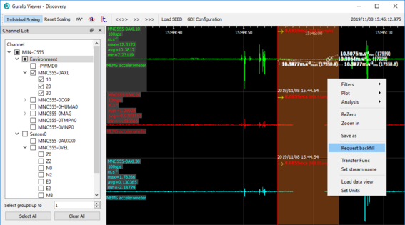
The gaps are backfilled automatically for all the streams selected, if the requested data is available in the microSD card.
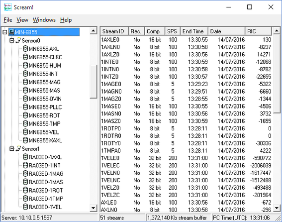
4.3.2 Using Scream!
Data from the Minimus and attached sensors can also be viewed and analysed using Güralp's Scream! Software.
For full usage information on Scream!, please refer to the on-line Güralp manual MAN-SWA-0001.
In Scream!’s Network Control window, add a UDP or TCP Server using the address reported under “LAN Address” in Discovery’s main window (as described in section 4.2).

Right-click on the newly-added server and select GCFSEND:B (or Connect) from the context menu. This sends a command to the Minimus to start data transmission. Once the GCFSEND:B (or Connect) command has been issued, the instruments and their associated streams should begin to appear in Scream!’s main window.
To configure the Minimus, double-click on its entry to open its web page.
Note: If stream recording is enabled, make sure that the file-name format in Scream! (on the Files tab of the File→Setup dialogue) is set to
YYYY\YYYYMM\YYYYMMDD\I_A_YYYYMMDD_HHNN
in order to prevent file names conflicting. More information can be found in Scream! manual MAN-SWA-0001 available on the Güralp website.