Chapter 6. WaveView windows

The most commonly used features of Scream! are accessed through WaveView windows. You can open as many WaveView windows as you like, on any combination of streams; the same stream can be part of several WaveView windows at once, at several different scales.

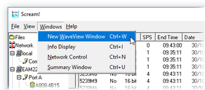
To open a WaveView window from Scream!'s Main Window, either:

• select Window → New WaveView Window… from the main menu;

  

• double-click on a stream ID in the streams list;

• right-click on a stream in the list and select View; or

• make a selection of streams and double-click the selection or key :

  • To select a range of adjacent streams, left-click ( ) on the first and then + on the last.

  • To select a non-adjacent set of streams, left-click ( ) on the first and then + on each additional stream.

You can add additional streams to the WaveView window by selecting them from the streams list and dragging the selection into the WaveView window, or by dragging them from other WaveView windows. Dragging with held down will copy the stream from one window to another; otherwise, the stream will be moved to the new window.

If you are running Scream! in real-time mode, and you double-click on a GCF file to view it (or open the Scream! viewer in some other way), you will have both real-time and “view” windows open. In this case, you can drag streams from real-time windows to other real-time windows, but not from these to view windows, or from view windows to other view windows. This is because the windows are handled by different instances of the Scream! program.

You can also drag streams within a WaveView window to reorder them. You will need to drag from the panel on the left, since dragging across the window will zoom in; see below.

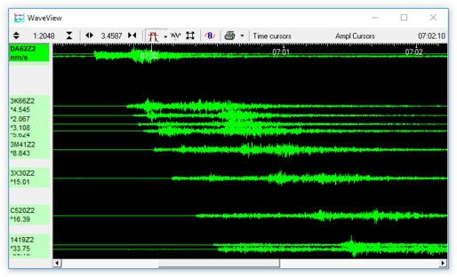
To the left of the stream display is a panel identifying the stream by its System ID and Stream ID, or by another label if you have set one (see section 6.4.2). If calibration values have been supplied (see section 5.7), the units of measurement will also be shown. If there is insufficient space, this text can become small or be omitted entirely. In this case, you can resize the panel by dragging its right-hand edge across the WaveView window, as shown in the illustration below. You can also hide the panel completely by dragging its right-hand edge to the left of the WaveView window.

If you have several WaveView windows open, the Windows menu in Scream!'s Main Window allows you quickly to bring focus to any of them. This is particularly useful if you have given the windows labels, as described in section 6.1.8:

6.1 Window functions

Above the stream display is a toolbar, containing icons which act on all of the streams within the window.

On the right of the toolbar, the time and date is displayed (when space is available). This is the time corresponding to the right-edge of the stream display window. Right-clicking on the date will toggle between displaying the date in year/month/day format and year/Julian-day format.

6.1.1  Zooming in and out

To zoom in and out vertically, either:

• click the vertical scale icons at the top of the window;

• use your mouse wheel ( ); or

• left- or right-click on the number itself.

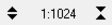
The current zoom factor is shown between the icons, as a ratio of pixels to counts. Zooming in and out affects every stream in the window.

To zoom in and out horizontally, either:

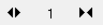
• click the horizontal scale icons ;

• hold down the shift-key whilst turning your mouse wheel ( + );

• left- or right-click on the number itself; or

• select the data by left-clicking and dragging the mouse. Release the mouse and select "Zoom In" from the context menu.

The current zoom factor is shown between the icons, in pixels per second. To convert to pixels per sample, divide the zoom factor by the sample rate for the stream. Where several samples are shown in a single horizontal pixel-width, a vertical line is plotted between the lowest and the highest sample values.

If you have a large window which takes some time to scroll, especially at a high horizontal zoom factor, Scream! may not be able to finish drawing new data before it needs to scroll again. If this happens, Scream! will delay scrolling until it can display in real time once more. To prevent this, decrease the time scale.

If you have paused the window with the icon ( when paused), you can zoom into an area of interest by dragging a rectangle across the streams. While you are dragging, Scream! displays the time span in the top right corner of the rectangle, and the number of counts in the bottom left corner. You can drag across one stream, or several; the resulting window will still include all streams.

Whilst the window is paused, you can also adjust the start and end times of the view by dragging the ends of the horizontal scroll bar button, at the bottom of the window.

6.1.2  Making measurements

Click the Time Cursors or Ampl Cursors button to display a pair of horizontal (time) or vertical (amplitude) cursors. Each cursor has a square at one end, which can be dragged across the WaveView window to measure features. If two cursors coincide, you will only be able to see the squares.

The distance between the cursors replaces the labels of the Time Cursors or Ampl Cursors button, in seconds and Hertz or counts. You can have both vertical and horizontal cursors active at the same time. Because the limit of accuracy of the cursors is one pixel, you should zoom in to the range of interest for greater accuracy.

The Ampl Cursors measure distances in counts according to the current zoom settings. However, if you have applied a scaling factor to an individual stream (see below), the Ampl Cursors do not take this scaling into account, so the measured distance will no longer be in digitiser counts; they will be in the scaled units of the stream.

To obtain the true value in counts, divide the value displayed in the Ampl Cursors icon by the scale factor for that stream, as displayed beneath its ID on the left-hand panel.

If a stream is shown with a physical unit (e.g. nm s-1), Scream! has scaled it so that the Ampl Cursors display a value in that unit. To do this, Scream! needs to know the calibration values - i.e. the sensitivities of your digitiser and instrument (see section 5.7).

It is also possible to take absolute measurements. The values obtained in this way are affected by any offset in place, as described in section 6.2.4, so these should be zeroed before you start. You can use the + keyboard shortcut to set the offset of every stream to zero. If you wish to reset the offset of a single stream to zero, hover the mouse over its lane and use the keyboard shortcut.

Zeroing an offset may cause the stream to move vertically such that it is no longer in its lane or even visible in the WaveView window. You can bring the waveform back into view by decreasing the amplitude, using the rightmost of the vertical scale icons at the top of the window or by scrolling the mouse wheel downwards ( ).

Once you have removed the offsets, you can measure detailed, absolute sample values, by holding whilst performing a click-&-drag action. A hint box will display the exact time of the sample and its value. This is always displayed in counts but values in physical units are also given if calibration info is loaded (see section 5.7). If the time scale is zoomed out such that multiple samples are on the same pixel, the maximum and minimum values for that pixel will be displayed:

6.1.3  Printing

To print the data currently being displayed in the WaveView window, click on the Print icon . Scream! will use the current default printer settings to print a full page view of the window, using the current amplitude and time scaling, filtering and other display options. You can print at any time, in either real-time or paused mode.

Extra print options are available in the drop-down menu of the Print icon:

To print the same data in black and white (on a colour or grey-scale printer), click on the arrow beside the Print icon and select Page Print (monochrome) from the drop-down menu. Black and white output is more suitable for copying or faxing.

You can also set up Scream! to print automatically, or send data directly to a connected plotter. For full details on the printing options available in Scream!, see Chapter 12.

6.1.4 Selecting data

Data can be selected from WaveView windows for use in a number of situations, including saving, processing and helping design filter responses.

It is sometimes helpful to pause the window before selecting data, as described in section 6.1.6. It is not, however, necessary.

Data selections can encompass one, two or more streams but the start and end times of the selection are the same across all streams.

When selecting from more than two streams, the streams must be adjacent in the WaveView window and the order in which the streams are presented is always top to bottom. If you need a different order, you can drag individual streams up and down the WaveView window to re-order them, or duplicate the entire window (keyboard shortcut + ) and delete any unwanted streams. When selecting from exactly two streams, you can choose the order.

6.1.4.1 Selecting data from one stream or several adjacent streams

To select data from one stream or several adjacent streams, hold down the Shift key ( ), click at the desired start-time in the first stream and then, while still holding the Shift key, drag to the desired end-time in the last stream:

The number of samples selected is shown at the top left of the selection.

If the region you have selected is entirely filled with contiguous data, the selection is shown as a solid block. If there are gaps or overlaps in any stream, the selection is shown in a hatched style:

6.1.4.2 Selecting data from exactly two streams

Select data from two (possibly non-adjacent) streams by holding down the Control key ( ), clicking at the desired start-time in the first stream and then, while still holding down the Control key, dragging to the desired end-time in the second stream:

The number of samples selected is shown at the top left of the selection.

6.1.5 Filtering

Clicking the Filter icon (or when selected) makes Scream! apply a filter to each of the displayed streams. Click the icon again to disable the filter.

Scream! can be configured to apply different filters to each WaveView window. To select the filter, click on the arrow beside the Filter icon. A drop-down menu will appear.:

From this menu:

• Select Default filter to apply Scream's built-in FIR bandpass filter. The properties of this filter depend on the sample rate of the stream. Data at 1 or 2 samples per second are filtered with a 10 – 30 second pass-band, whilst data at other sample rates are filtered with corner frequencies at 0.1 and 0.9 times the Nyquist frequency of the stream. For example, the pass band for the filter applied to a stream at 100 samples per second will be 5 – 45 Hz.

• Select Custom filter to activate the filter you have designed. If you have not designed a filter, a 10 – 30 second pass band filter will be used for all sample rates.

• Select Design… to open the Filter Design window (see section 6.3).

• If you have saved some filter designs as presets (see section 6.3.5), they will be listed below Design…. Select an entry to switch to a Custom filter with these settings.

• If you have saved some filter designs as presets, a Delete preset sub-menu will also appear. Select an entry in this sub-menu to delete that filter definition.

6.1.6  Paused mode

Click the Pause icon (or when selected) or use the shortcut key to stop the window scrolling. If new blocks arrive which contain data from the time period displayed, Scream! will add them to the window.

Whilst a window is paused, you can scroll the waveform to the left or right to view all the data that Scream! has in memory. This can be done dragging the horizontal scroll bar at the bottom of the window to the left or right or by turning the mouse wheel while holding down the key.

You can also drag either edge of the horizontal scroll-bar in order to change the degree of zoom, as shown below:

All of the following options are also available without pausing the display but it is often easier to pause the window first. You can:

• Use the mouse-wheel ( )to zoom in and out to examine features in the data. Hold the Shift key while using the mouse wheel ( + ) to zoom in and out in the time series, centred on the mouse position.

• Select data as described in section 6.1.4.

• Clear any selections and re-draw the display by keying . (This also cancels any stream-positioning functions and recomputes the display cache so it can be a little slow when very large amounts of data are displayed.)

• Use data in a filter design by selecting data from a single stream and choosing Use in Filter Design… from the pop-up menu. See section 6.3 for details.

• Pass data to a Scream! extension by selecting data as described in section 6.1.4 and choosing the required extension from the pop-up menu. See Chapter 14 for more details.

• Save data to a file by selecting data as described in section 6.1.4 and choosing Save…:

  

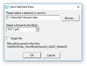
  Select the directory and format for the file, and click to save the data with one file for each stream (using the format shown).

  Some formats support multiple streams per file. For these formats, you can select Single File to combine the streams. See section 11.1.1 for details about the various file formats.

Click the Pause icon ( ) again (or key ) to return to real-time mode. If you have changed the zoom settings, the window will return to its previous state, with the window once more following the real-time data.

6.1.7  Other icons

Click the Block Boundaries icon to display a dotted line at the end of every GCF block displayed in the window:

The number beside each line is the number of bits used to store each sample in the block. A fixed-length GCF block with 8-bit samples (which can encode differences from -128 to +127) can store 4 times as many samples as a block using 32 bits for each one (encoding differences larger than two billion counts). Clicking the icon again removes the block markers. Block markers can also show icons for re-boots ( ) and re-syncs ( ) when reports of these are detected in the associated status stream.

Click the Null Offsets icon or use the + keyboard shortcut to centre each stream vertically in its lane. This is done by adjusting the offsets such that the mean value of the waveform (over the time period displayed in the window) is zero. If you do not want a particular stream to be zeroed when you click this icon, right-click on the stream beforehand and select Locked Offset from the context menu. If you wish to null the offset of a single stream, move the mouse into its lane and use the keyboard shortcut.

When Scream! is used as a data viewer, the Pause icon ( ) is replaced with the Restore View icon: . Click this icon to reset the time and amplitude zoom settings to their initial values - i.e. to display the entire selected data set within the window.

6.1.8  Context menu

Right-clicking inside a WaveView window brings up a context-sensitive menu in two sections, divided by a horizontal line:

The upper section of this menu contains options which affect a particular stream. These are described in section 6.2. Options in the lower section affect the whole window and are described here.

Select Background Colour… to change the background colour for the window.

Select Show Lane Lines to toggle the drawing of the lane boundaries, zero reference lines and time reference lines:

Select Label… to change the title of the window. This also changes the name of the window's entry in Scream's Windows menu and the name that is used on print-outs (see Chapter 12).

Select Clear Window to remove all streams from the window. This does not remove the streams from memory; you can retrieve them by dragging from Scream's Main Window onto the now-empty WaveView window.

Select No Caption to remove the title decoration and toolbar from the window. To maximise the screen area occupied by streams, first maximise the WaveView window, then choose No Caption. You can still use the mouse wheel or keyboard shortcuts (see Chapter 15) to perform the actions of icons on the toolbar.

Select Duplicate to open a new WaveView window identical to the current one. (If you have renamed a stream using Stream Name Mapping, the new window will use the new name.)

The Axis Spacing sub-menu has a number of options:

• Normal ( keyboard shortcut) – the default, even spacing. This command cancels any of the stream-positioning functions listed below and recomputes the display cache. This may cause a small delay if enormous amounts of data are displayed.

• Overlay streams ( keyboard shortcut) - to draw all visible streams in the middle of the window, overlaid one on top of another. This is useful if you want to compare event records from several instruments in an array. Key to cancel and return to the normal stream spacing.

• Depth ( keyboard shortcut) – if the calvals (see section 5.7) contains a depth= entry for every stream in the window, this option will space the traces vertically, relative to the depth value. This can be useful for vertical seismic profiling "strings": i.e. when several instruments occupy the same borehole. Key to cancel and return to the normal stream spacing.

• Distance From Point ( keyboard shortcut) – available if all instruments have Latitude/Longitude coordinates set in the calvals (see section 5.7), and you have specified a Set Point ( + keyboard shortcut). This is useful for aligning earthquake phase arrivals. Key to cancel and return to the normal stream spacing.

  

• Station map in Google Earth - this option is available if all instruments have Latitude/Longitude coordinates set in the calvals (see section 5.7). Selecting this option creates a .kml file mapping the station locations and calls Google Earth to view the file.

The Sort by sub-menu offers the following options:

2

• Stream ID - Sort by Stream ID. Where duplicate Stream IDs exist, maintain the previous sort order.

• Component - Vertical components (ending Zx), followed by Nx and Ex components, then Mux channels Mx. Within a component type, sort by the first four characters of the Stream ID.

• Instrument - Sort by the first four characters of the Stream ID. Within an instrument, sort by tap, then by component.

• Sample Rate - Sort by sample rate, highest to lowest. Within a sample rate, sort as Instrument.

• Tap - Sort by tap (the last character of the Stream ID). Within a tap, sort by instrument, then by component.

• System ID - Sort by System ID. Within a System ID, sort as per instrument, described above.

• Location - this option is only available if all instruments have Latitude/Longitude coordinates set in the calvals (see section 5.7). It displays a sub-menu:

  

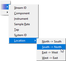
  At any one location, sorting is as per component, described above.

The Spectrogram size sub-menu allows the user to change the vertical size - and, hence, resolution - of the spectrograms in the current WaveView window..

When the sub-menu is displayed the following key-strokes can also be used to select a size:

• - set the size to 16 pixels

• - set the size to 32 pixels

• - set the size to 64 pixels

• - set the size to 128 pixels

• - set the size to 256 pixels

• - set the size to 512 pixels

• - set the size to 1024 pixels

This allows the spectrogram size to be changed entirely from the keyboard with a sequence like .

When you first enable spectrograms, the initial height of each is determined from the setting in the Display options pane of the Setup window. See section 6.4.1 for details.

See section 6.2.5 for details of spectrogram operations.

6.2 Stream functions

Actions can be performed on streams in a WaveView window using the context-sensitive menu, which appears when you right-click in the window.

Each stream has its own “focus lane”, although high zoom factors may make the trace extend outside the lane. The background colours have been altered in the window below to make the extents of the lanes visible. Right-clicking in any focus lane bring up the context menu for the associated stream.

If you have selected Overlay Streams for the window (as below), the focus lanes are still present, even though the streams are no longer drawn inside them. Right-clicking in the window anywhere to the right of a stream identifier will still bring up the context menu for that stream.

The context menu is divided into two by a horizontal line.

Items in the top section (above the divider line) apply to the individual stream and are described in the following section. Items below the divider line apply to all streams in the current WaveView window and are described in section 6.1.8.

6.2.1  Identifying streams

Every stream is identified in its icon in the left-hand panel. For more details, right-click on the stream. The topmost option in the context menu displays the full network path to the instrument, including its System ID and Stream ID:

Here, a vertical stream (Z2) from a digitiser with the System ID BHCH2 and Serial Number HONE has a mapped name of BHCH2-GSL_Z2 (see section 6.4.2). Right-clicking on the stream shows that the true Stream ID is BHCH2-HONEZ2, and that it originates from port Com24 on a system called JURAND. The data from JURAND have been forwarded by another system called BANFF.

6.2.2  Changing the appearance of streams

To change the colour of a stream's trace, right-click on the stream in the WaveView window and choose Colour…. Select the colour you want to use and click .

There are two further options for defining trace colours:

• You can set the default colour for each component (Z, N, E, and X) from the Display tab of the File → Setup… dialogue. See section 6.4.1 for more details.

• You can set up Scream! to use particular colours automatically according to the name of the stream, and to label them differently in the WaveView window. See section 6.4.2 for more details.

6.2.3  Scaling streams

To scale an individual stream, right-click on it and select Scale…:

Enter the new scale factor and click . You can scale whole instruments at a time by ticking the all […] components in this window box. This overrides any previous scale-factor active for those streams. Select “all streams in this window” to set the scaling using the value entered for all streams.

If you have configured Scream! to scale streams to physical units, this box will display the scale factor that Scream! is using. If you entered a different scale factor, it will override the factor Scream! has chosen. To return to physical units, in the scaling box, enter the word “auto”. You can also apply relative scaling by entering * and / operators. For example, entering a scaling of *2 will double the existing scale factor.

You can also type in the name of another stream that is in the same WaveView window. The selected stream will then be scaled such that the maximum/minimum range matches that of the stream you typed in.

To perform a one-time auto-scale of all streams so that the maximum/minimum is the same for all of the displayed data, right-click on the stream you want to be the reference,, and select the Scale others to match option ( + keyboard shortcut).

The keyboard shortcut will reset the active stream to a scale factor of 1. To reset all streams in the WaveView window, key + .

6.2.4  Viewing offsets, ranges and averages: Details windows

To see the mean, range, average and RMS values for a stream, right-click on it and select Details…. A small window will appear beside the stream giving the current offset, mean, maximum and minimum values for the data in the window, together with the Diff (the difference between the minimum and maximum values). The values are scaled according to the current scale-factor for the stream, or to any physical unit you have selected.

To alter the vertical offset of a stream, type a new value (in counts) into the Offset box and press . You can do this even if the stream has its offset locked (via the WaveView window's right-click context menu). The offset is changed for the current WaveView window only but it does affect any absolute measurements taken, as described in section 6.1.2.

If you move a WaveView window, all its Details windows will move with it. You can change their relative position by dragging the title bar of each Details window.

Whilst the Details window is open, the mean value is displayed on the WaveView window as a dotted horizontal line, whilst the maximum and minimum values are displayed as solid lines.

You can also change the offset of a stream with the keyboard. With the mouse over the Details window, pressing the and arrow keys moves the current stream up or down by one pixel, whilst and move the stream by the height of one “lane”. This feature lets you compare streams by placing one directly on top of another. The lane used for selecting the streams stays the same.

While the details window is open, the keyboard shortcut can be used to null the offset of the associated stream, centring the mean of the stream vertically in its lane.

(When the details window is closed, the key only nulls the offset of the active stream: to null all active offsets in the current WaveView window, use + .)

6.2.5  Spectrogram

Scream! can perform real-time spectral analysis on incoming data. To enable this feature, right-click on the stream of interest in the WaveView window and choose Spectrogram from the pop-up menu or use the keyboard shortcut. This displays or hides the spectrogram on a stream-by-stream basis. You can use the keyboard shortcut + to display/hide all spectrograms at once.

6.2.5.1 Interpretation

The vertical axis of the spectrogram is linear, with the Nyquist frequency (which, by definition, is equal to half the sample rate) at the top and 0 Hz (DC) at the bottom. The colouring is logarithmic, giving a large total range whilst retaining sensitivity at low signal levels. Red represents the highest amplitudes and deep purple the lowest. Loosely speaking, the "hotter" the colour looks, the higher the amplitude.

6.2.5.2 Height

The height of each spectrogram in any given WaveView window is the same. When you first enable spectrograms, the initial height of each (in pixels) is determined from the setting in the Display options pane of the Setup window.

Once spectrograms have been enabled in an individual WaveView window, their height can be changed by right-clicking in the window and using the context menu - see section 6.1.8 for details.

6.2.5.3 Contrast

The colour contrast of any individual spectrogram can be changed by hovering the mouse over it and using the and shortcut keys. Hold at the same time in order to apply the changes to all spectrograms in the current WaveView window.

This works by applying a ×2 or ÷2 scale factor to the stream data before applying the Fast Fourier Transform calculations. You can achieve the same effect by changing the scale factor of the stream (see section 6.2.3), although this would also affect the size of the trace in the display.

6.2.5.4 Zooming in

The spectrogram supports zooming in to particular frequencies by holding down the left mouse button while dragging a selection across the frequency scale:

To apply the same zoom factor to all spectrograms in the current WaveView window, hold at the same time.

To zoom out to the previous setting, right-click on the frequency scale (holding , if desired, to apply the change to all spectrograms).

6.2.5.5 Example

The example below shows data from a 5TD which is sensing a signal of approximately 40 Hz, as shown in the green trace at the top.

The Red trace shows:

• the N/S component, with the spectrogram zoomed in once; and

• the blue trace where the spectrogram is zoomed in again, to the 39-40.5 Hz region.

On closer inspection, it can be seen that the signal frequency is changing over time, which was not apparent from the un-zoomed green trace. This could be a valuable diagnostic indication when trying to understand the source of the signal.

6.3 Filtering

Scream! can apply filters to your data before displaying them in a WaveView window. This feature allows you to eliminate frequency bands which contain unwanted noise and focus on frequency bands which contain data of interest. It can make a dramatic difference to the visibility of teleseisms in noisy data.

To apply or remove the filter, click the button or use the shortcut key. Both act as toggles, turning the filter alternately on and off.

The properties of the default filter depend on the sample rate of the stream. Data at 1 or 2 samples per second are filtered with a 10 – 30 second pass-band, whilst data at other sample rates are filtered with corner frequencies at 0.1 and 0.9 times the Nyquist frequency of the stream. For example, the pass band for the filter applied to a stream at 100 samples per second will be 5 – 45 Hz.

In addition to the default filter, a custom filter response can be created. The Filter Design window allows you apply low-pass, high-pass or band-pass filters. Each WaveView window can have its own Filter Design settings.

Filter designs can be saved (with useful, mnemonic names) and retrieved.

To open the Filter Design window, click on the arrow to the right of the Filter icon and select Design… from the drop-down menu:

Alternatively, use the + keyboard shortcut.

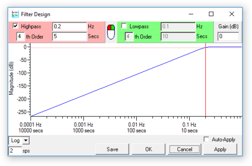
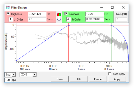
The Filter Design window opens:

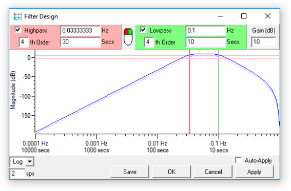
From top to bottom, the window contains

• the parameters of the current high-pass (red) and low-pass (green) filter in numerical form,

• a graph of the response of the current filter, showing the –3 dB level and corner frequencies,

• (at bottom left) display settings for the graph, and

• (at bottom right) control buttons for the window.

6.3.1 Filter parameters

The filter parameters are shown at the top of the Filter Design window.

• Select Highpass to switch on the high-pass filter, and enter the value of the corner frequency required in either the Hz or the Secs (seconds) box. You are not allowed to enter a value of 0 in either box.

  Alternatively, change the corner frequency by clicking and dragging across the graph with the left mouse button . If the low-pass filter is active, and you click to the right of the low-pass corner, both frequencies will be moved.

  If the frequency you want is not shown in the window, it may be above the Nyquist frequency for the currently-selected sample rate. Change the value in the n sps box at the bottom left and try again.

  Change the order of the filter by entering a number in the nth Order box. If the cursor is in this box, pressing the and keys will alter the order by one in either direction.

  

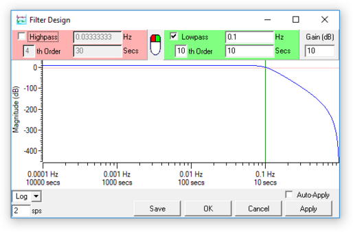
• Select Lowpass to switch on the low-pass filter, and enter the value of the corner frequency required in either the Hz or the Secs (seconds) box.

  

  Alternatively, change the corner frequency by clicking on the graph with the right mouse button . If the high-pass filter is active, and you click to the left of the high-pass corner, both frequencies will be moved.

  Change the order of the filter by entering a number in the nth Order box.

• To create a band-pass filter, select both Highpass and Lowpass. Enter values into the text boxes, or click in the graph with the left and right mouse buttons to set the two corner frequencies.

  

  When both filters are active, the individual filter curves are shown on the graph in light blue.

• Enter a value in the Gain (dB) box to change the gain of the filter.

  In the example above, the overall gain of the band-pass filter has been set to 10 dB. This is done by applying a 5 dB gain to each of the component filters. As a result, the light blue traces appear 5 dB below the dark blue trace.

6.3.2 Viewing spectra

You can overlay the power spectra of up to two streams on the frequency graph. This is intended to help you design filters for specific events by focussing on the frequencies at which the event has significantly more energy than the background noise.

To design a filter for a specific event:

• View the relevant stream in a WaveView window. If the window is not paused, it may be useful to pause it. Locate a time period where the stream is quiet.

• Shift-drag ( + ) to select the (single) stream across this quiet time range. Choose Use in Filter Design… from the context menu.

  

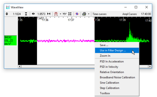
  Note: If you do not see the Use in Filter Design… option, check that only one stream is selected.

  The Filter Design window will appear, with the spectrum of the background noise overlaid in grey.

  

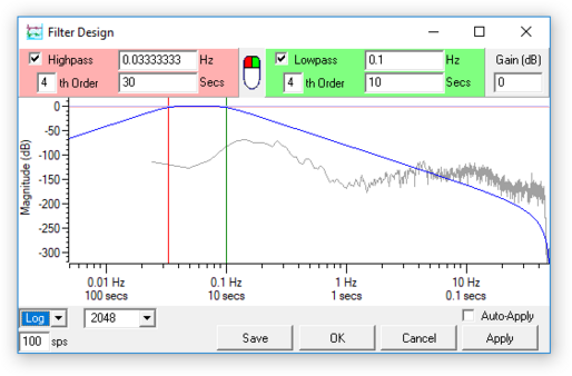
• Leaving the Filter Design window open, switch to the WaveView window and view the event of interest.

• Shift-drag ( + ) to select data from the same stream during the event. Choose Use in Filter Design… from the drop-down menu.

  

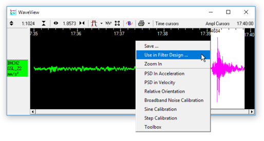
• A dialogue box will open asking you if you want to replace the previous spectrum or add to it:

  

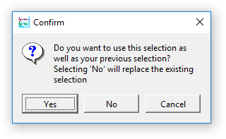
  Click . The spectrum of the event will be overlaid onto the background noise spectrum, in a lighter shade.

  You can now click in the graph to move the filter's corner frequencies to suit the event:

  

  The drawing of the mouse ( ) reminds you that the left mouse button controls the high-pass filter and the right-mouse button controls the low-pass filter.

• If you want to view the spectrum of a different event, follow steps 3 – 4, choosing when you are asked if you want to overlay the spectra. The old event spectrum will be replaced with the new one.

• If you want to change the background spectrum, follow steps 1 – 2 and choose when you are asked if you want to overlay the spectra. The old event spectrum will be erased, and the background spectrum will be replaced with the new one. Now follow steps 3 – 5 to overlay the spectrum of a different event, as desired.

6.3.3 Display options

The icons at the bottom left of the Filter Design window change the properties of the graph.

• The Log/Lin selection box allows you to choose a logarithmic or linear time axis. (The magnitude axis is always displayed in dB, and is therefore always logarithmic.)

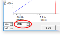
• Enter a value in the n sps box to display a frequency/period range suitable for streams at that rate. The graph displays a five-decade frequency range, up to the Nyquist frequency (i.e. half of the entered sample rate).

• When power spectra are being displayed on the graph, there is an additional selection box to the right of the Log/Lin icon.

  The power spectrum calculation uses the Welch averaging periodogram algorithm. This algorithm produces frequency graphs by splitting the range into windows of a certain size. You can alter the size of window used by changing the value in this selection box.

  

  Using a smaller window size produces a smoother graph, at the expense of losing information about lower frequencies. To examine lower frequencies, you will need to increase the window size; however, doing this will increase the noise visible at high frequency.

6.3.4 Using your filter

When you are happy with your filter design:

• Click to apply the filter to the WaveView window and close the Filter Design window.

• Alternatively, click to apply the filter and leave the Filter Design window open.

Ticking the Auto-Apply check-box makes the Filter Design window apply immediately any changes you make to the filter. Since applying a filter may take some time, you should not tick Auto-Apply if you are viewing a large amount of data. However, it can be very useful to interactively see the effects of changing the high-pass and low-pass corner frequencies, when dragging around with the mouse.

6.3.5 Pre-sets

If you have designed one or more filters that you would like to use repeatedly, you can save them as presets. To save the currently-active filter into Scream!'s configuration file, click and enter a name for the filter:

You can now select that filter, by name, from the drop-down menu next to the WaveView window's Filter icon. All of your saved presets will be listed under the Design… entry.

The menu is also extended to include a Delete preset sub-menu, from which you can delete any of your saved filter definitions.

To modify an existing preset, first load it and then delete the definition. Revisit the design window, make the modifications that you want and then save the new version using the same name.

6.4 Display options

There are a number of Scream! set-up options which affect how WaveView windows are displayed.

6.4.1  Display set-up

To change default display options for new WaveView windows, choose File → Setup… from the main menu and click on the Display tab.

Stream Buffering : You can change the size of Scream's stream buffer by altering the value and unit in these boxes. Scream! will discard any data older than this. If you want to record data to your computer's hard disk, you should use the Recording and Files panels; when you enable recording on a stream, any data in the stream buffer will be included in the recorded files. Scream! can also play back recorded GCF files (see Chapter 11).

Status Font : Click to change the font used in status stream display windows. The change comes into effect on new and existing Status windows as soon as you click click  or  .

WaveView Defaults : Allows you to take the default properties for new WaveView windows from a window already on the screen. Click  and then click on the window you wish to copy. When you click  or  , new WaveView windows will have the same horizontal zoom factor, filter and block boundary options, background colour, and time/amplitude cursor state as are currently in place on that window. The vertical zoom factor is used only for new, blank WaveView windows, since Scream! automatically chooses a suitable factor if it can.

Colour-coded Components : When this box is ticked, Scream! will look for stream names ending Zn, Nn, En or Xn and automatically display them in the colours shown. To change the default colours, click on the boxes. Other streams are assigned a colour in rotation as they arrive. To define more specific colour defaults, you can use stream mapping (see below).

Spectrogram : Alter this value to change the default height of spectrograms displayed in WaveView windows, in pixels. When you click  or  , newly-drawn spectrograms in all WaveView windows will use the new height. Pressing will cause a WaveView window to be redrawn, as will resizing it, changing the zoom factor or using other buttons on the toolbar. Moving a window, or obscuring it and then revealing it, may or may not cause a redraw, depending on your operating system.

Units : Scream! can automatically scale new WaveView windows to physical displacement, velocity, acceleration units using sensitivity information you provide (see section 5.7). To enable this feature, first edit the calibration values for your digitiser, then select a suitable unit from the Displacement, Velocity, or Acceleration drop-down lists.

Once you have done this, streams from the digitiser will be scaled automatically. Other instruments will default to displaying in counts.

A simple linear scaling algorithm is used, which does not take into account the response profile of the instrument, although where the instrument has a flat response in the pass-band, it is normally a sufficient approximation. For accelerometers, this is usually sufficient to be useful.

6.4.2  Stream mapping

You can tell Scream! to look for streams with a particular Stream ID, and to display them in WaveView windows with their own colour and label. This is configured from the set-up window. As with all set-up options, Scream! will remember any mappings you create in the scream.ini file and restore them next time you run the program.

To create a new stream mapping:

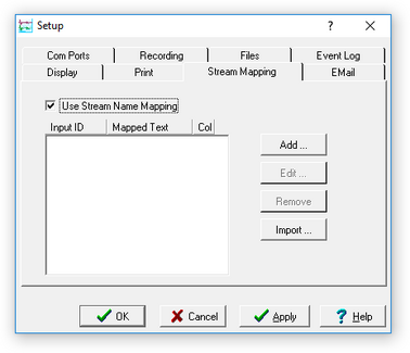
• From Scream!'s Main Window, choose File → Setup…. Switch to the Stream Mapping tab.

• Tick Use Stream Name Mapping. The pane will change to show the new options:

  

• Click and fill in the Stream ID you want to change, the new label and colour:

  

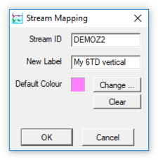
  The label can be any length, but may not contain any of the characters

  \ / : * ? " < > |

  because these characters are not allowed in DOS or Windows file-names.

• Click . In this example, new WaveView windows containing the DEMOZ2 stream will now automatically show it in the new colour, and with the label My 6TD vertical. The new label is also used in the Main Window, on print-outs and in the file-names of recorded data streams (if your format specifier includes the mapped Stream ID). Identifiers inside exported files will still use the original Stream ID.

  WaveView windows which are already open will not change until they are refreshed (e.g. by resizing or zooming them, or by pressing ).

You can edit an existing mapping by double-clicking on its entry in the table, or by selecting it and clicking Edit…. To change the default colour only, click the colour panel under Col in the table.

To delete a stream name mapping, select it and click .

Clicking enables you to import a scream.ini file from another Scream! installation and extract the mappings from it. This is useful when you want to use a standard set of names and colours for several Scream! installations.